PiVR has been developed by David Tadres and Matthieu Louis (Louis Lab).
7. Tools
Important
The software has different functionality if run on a Raspberry Pi as compared to any other PC. This manual is for the PC (Windows, MacOS and Linux if not run on a Raspberry Pi) version of the software
7.1. The Menubar
To select a different window use the Menu Bar at the top of the window
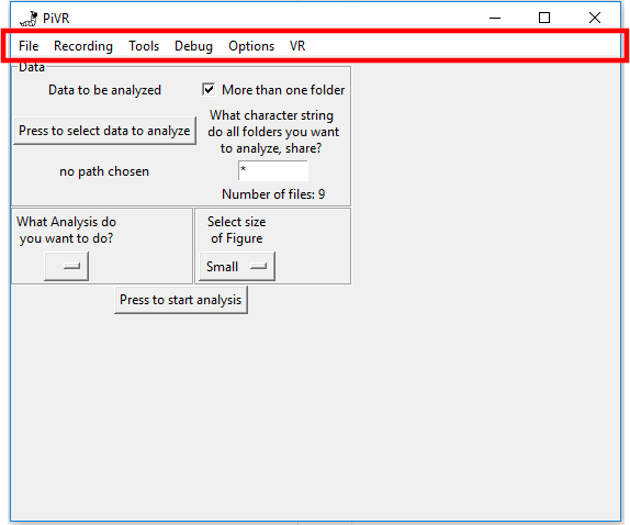
7.2. The Analysis Menu
The Analysis Menu lets you choose a folder (either with one experiment or a folder containing several experiments) and run different analyses.
To analyze an experiment (or several) first press the “Press to select data to analyze” button on the top left. Select a folder. You may:
Select a single experiment. In that case you must uncheck the button on the right next to “More than one folder”.
Select a folder containing several experiments. If this folder only contains folders you want to apply the same analysis, you do not have to do anything. If there are other files or folders, please indicate a commonality between all the folders in the entry field below. This can be the date (e.g. 2019) a genotype (e.g. Or42a) or..
The “Number of files” below the entry field indicates how many files and folders in the folder you selected is taken into account if the current input is used.
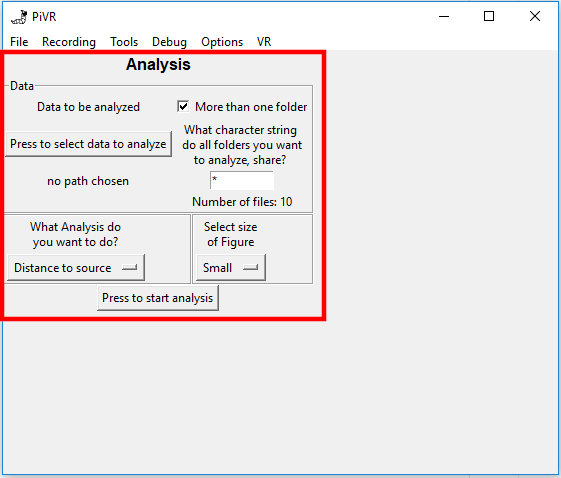
Next, select what analysis you want to do. Currently there are several options:
7.2.1. Distance to source
If you are interested in the distance the animal has to a point in its environment try this option.
We used it in our publication to produce Figure 2D: A fruit fly larva behaving in an environment with a single odor source. We were interested in the distance to this odor source during the experiment.
To use this analysis program, you must have used the Tracking tab on PiVR or you must have recorded a Video or taken Full Frame Images with subsequent Post-Hoc Single Animal Analysis.
Important
If you want to use the multiple experiment options, please ensure that you have identical Framerates and identical Recording length
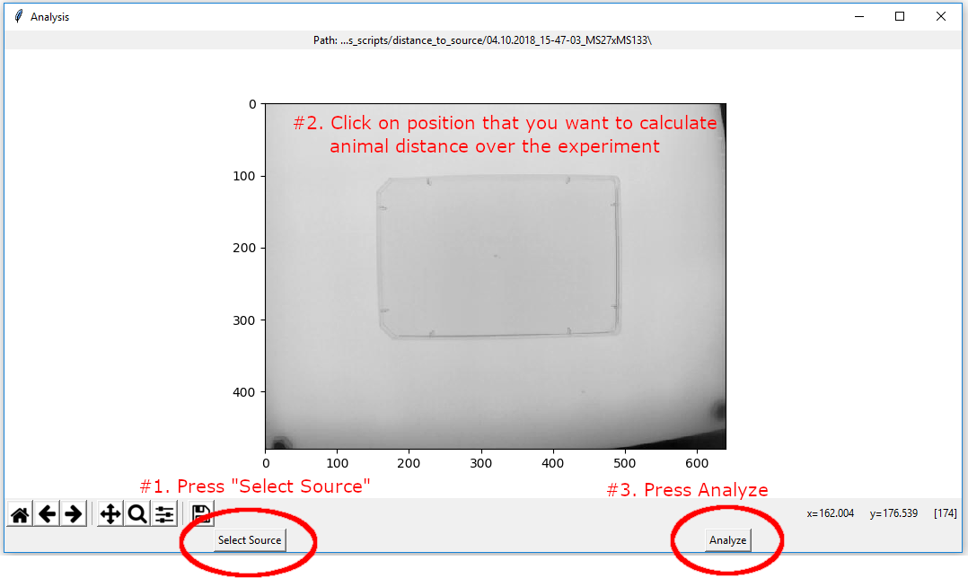
After selecting a folder and pressing “Press to start analysis” a popup will emerge that will ask you to “Select a source”. Do the following:
Press on the button that says “Select Source”
Click on the image where the “Source” is. In our case this would be an odor source roughly in the center of the dish. In your case it could be any single point
Once you are satisfied with the arrow placement, press “Analyze”
Once the analysis has finished you will find:
“distance_to_source.csv” in each experimental folder. This csv file contains the calculated distance to source in mm for each frame.
“Distance_to_source.png” in each experimental folder. This plot is intended to give a quick overview about the distance to source of this experiment.
If you have analyzed multiple experiments you will also find:
“all_distance_to_source.csv” in the parental folder. This file contains the calculated distance to source in mm for each frame (rows) for all the analyzed experiments (columns)
“Median_Distance_to_source.png” in the parental folder. This plot is intended to give a quick overview about the distance to source of all the analyzed experiments. Individual experiments are plotted in light grey and the median in red.
See here for actual code:
analysis_scripts.AnalysisDistanceToSource
7.2.2. Distance to source, VR
If you ran a virtual reality experiment with a single maximum point and you wish to calculate the distance to that point, try this option.
We used this analysis in our publication to produce Figure 2E: A fruit fly larva behaving in an virtual odor reality. We were interested in the distance to this virtual odor source during the experiment.
To use this analysis program, you must have used the Virtual Reality tab on PiVR.
Important
If you want to use the multiple experiment options, please ensure that you have identical Framerates and identical Recording length
After selecting a folder and pressing “Press to start analysis” the script will automatically read the virtual reality arena presented during the experiment and calculate the distance of the animal to the maximum point of stimulus intensity in the virtual reality.
Once the analysis has finished you will find:
“distance_to_VR_max.csv” in each experimental folder. This csv file contains the calculated distance to the maximum point of stimulus intensity in the virtual reality in mm for each frame.
“Distance_to_VR_max.png” in each experimental folder. This plot is intended to give a quick overview about the distance to source of this experiment.
If you have analyzed multiple experiments you will also find:
“all_distance_to_VR_max.csv” in the parental folder. This file contains the calculated distance to the maximum point of stimulus intensity in the virtual reality in mm for each frame (rows) for all the analyzed experiments (columns)
“Median_Distance_to_VR_max.png” in the parental folder. This plot is intended to give a quick overview about the distance to source of all the analyzed experiments. Individual experiments are plotted in light grey and the median in red.
See here for actual code:
analysis_scripts.AnalysisVRDistanceToSource
7.2.3. Single animal tracking (post-hoc)
If you have recorded image sequences or videos of single animals behaving and you wish to track their position, try this option.
While it works best if the PiVR Full Frame Recording or the PiVR Video recording option was used, the analysis program should be able to handle other image sequences and video files as well.
Important
Make sure that one experiment/trial is in one folder. For example, if you have recorded three videos, ‘Video_1.mp4’, ‘Video_2.mp4’ and ‘Video_3.mp4’ each video must be in its own folder (e.g. ‘Video_1.mp4’ goes into ‘Folder_1’, ‘Video_2.mp4’ goes into ‘Folder_2’ etc.),for the analysis software to work.
Once you press the ‘Press to start analysis’ button, the software will check whether it can find metadata in order to perform the tracking. If it does not find it, it will ask for user input. Specifically, it needs:
The frame rate the video/image sequence was recorded in.
How many pixels are one mm. The software will use the identical popup as on PiVR with the only difference being that you have to select a file with a known distance.
An estimate of the maximum animal speed. If unsure, it is better to overestimate the speed. If the tracking algorithm does not produce the desired result the maximum animal speed should be lowered.
An estimate of the maximum length of the animal. If unsure, it is better to overestimate the length. If the tracking algorithm does not produce the desired result, the maximum length should be lowered.
This tracking algorithm is identical to the tracking algorithm used for live tracking of the animal in PiVR.
The output is therefore almost identical to a tracking experiment run on PiVR. See here for an explanation.
The only two differences are:
You will find a file called “DATE_TIME_heuristics.csv” in the analyzed folder. This file contains useful information in order for you to define a new animal in “list_of_available_organisms .json”.
The “DATE_Time” for both the heuristics.csv and the data.csv indicate the time of the analysis NOT the time of recording the data.
7.2.4. Select analysis area (circle)
Usually animals are confined in a dish, for example a petri dish. If the animals are close to the border it can be difficult to get reliable data as the high contranst at the border can often lead to ‘jittery’ tracking. One solution is to discard all data where the animals are outside of a user defined area.
With v1.8.0. this idea has been implemented for a circular area. Select a folder containing many experiments (or just one folder, but then unselect the ‘More than one folder’ checkbox) and press ‘Press to start analysis’.
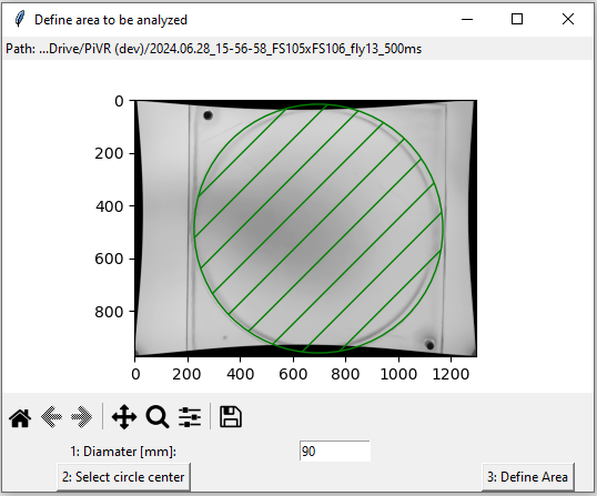
Then the following needs to be done for every experiment:
Select the diameter. This depends on px/mm to be correct. If you have data where this value is incorrect you can manually change it in ‘experiment_settings.json’.
Next, press the ‘Select circle center’ button and manually select the circle you want to use.
Finally, press ‘Define Area’ to continue to the next experiment.
This will add a new column in the data.csv file which indicates at which timepoints the animal was inside the user defined area
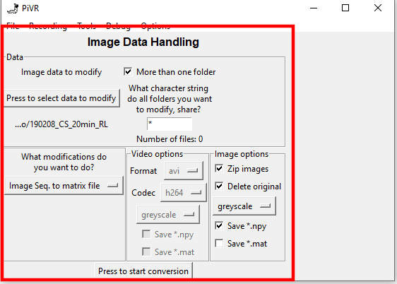
7.3. The Image Data Handling Menu
The Image Data Handling Menu lets you choose a folder (either with one experiment or a folder containing several experiments) and convert the image data.
To convert image data (either a series of full frame images or videos) first press the “Press to select data to modify” button on the top left. Select a folder. You may:
Select a single experiment/folder. In that case you must uncheck the button on the right next to “More than one folder”.
Select a folder containing several experiments. If this folder only contains you want to apply the same image data conversion, you do not have to do anything. If there are other files or folders, please indicate a commonality between all the folder in the entry field below. This can be the date (e.g. 2019) a genotype (e.g. Or42a) or…
The “Number of files” below the entry field indicates how many files and folders in the folder you selected will be taken into account if the current input is used.
Next, you have to choose the image conversion you want to perform using the dropdown menu under “What modifications do you want to do?” . Currently there are the following options:
7.3.1. Image Seq. to matrix
This is intended to be used after recording a series of images with the Full Frame Recording Option option of PiVR. The disadvantage of having a large number of single image files instead of one large file (with the identical size) is the time it takes the PC to read and write (e.g. copy, manipulate etc.) many single image files. This program will help you to “pack up” your image files. There are a variety of options you can choose from on the right side of the GUI:
Zip Images: If this checkbox is marked, the images will be zipped. You will find a zip file called ‘images.zip’ in the folder where the original images were located. The zip file is uncompressed - the goal here is to have one file instead of many single files, not to save disk space!
Delete Original: If this checkbox is marked, the script will delete all images that are considered to be part of the recorded image series. After zipping the images, it is useful to delete the original images as they will only make data handling slow, but: Make sure to only have this option on if at least one of the other options is selected, otherwise your data will be lost!
Greyscale/Color: This dropdown menu lets you choose whether you want the images to be saved in greyscale (standard, especially if a standard PiVR version is being used) or if the input colors are color images and you want the output to be saved as color images. Be careful with the color option, this has not been fully tested yet-.
Save *.npy: If this checkbox is marked, the script will save the images in a Numpy array. This can be very handy if you want to use python to run the downstream analysis of the data.
Save *.mat: If this checkbox is marked, the script will save the images in a Matlab like array. This can be very handy if you want to use Matlab to run downstream analysis of the data.
7.3.2. Video conversion
This is intended to be used after recording a video with the Video option of PiVR. Many users will find the h264 video file straight from PiVR inconvenient to work with, since: (1) Many video players (e.g. VLC) have problems decoding the video and (2) the metadata of the video seem to not always be correct.
Note
I found that the metadata of the videos recorded on the Raspberry Pi are not completely correct. For example, when reading a video file with the imageio module (using ffmpeg) the number of frames is given as “inf” and the framerate seems to be always at 25, even though the video was recorded at a different framerate. This script takes care of this bug by using the ‘experiment_settings .json’ file created when using PiVR to record a video.
There are several options available to define the desired output:
avi/mp4/None: If you want to watch the video, it is probably a good idea to convert the video either into avi or mp4 as your video player will be better able to handle these formats (and the metadata of this file will be correct, see above). If “None” is chosen, the video will not be converted.
h264/raw video: Besides the format, the codec can be a problem for some programs you want to open a video. Here, you can choose between the efficient h264 codec which will lead to very small file sizes and the raw video codec. The latter will lead to significantly larger video files! h264 is recommended!
Greyscale/Color: This dropdown menu, lets you choose whether you want the video to be in color (only works if original video is in color, of course) or converted to greyscale.
Save *.npy: If this checkbox is marked, the video will save each frame in a Numpy array. This can be very handy if you want to use python to run the downstream analysis of the data.
Note
Video encoding has been perfected over the years. Decompressing a video often leads to surprisingly large files, especially for long videos, or videos with a high framerate. If the uncompressed video is larger than your computer has RAM this script will most likely fail.
Save *.mat: If this checkbox is marked, the script will save the images in a Matlab like array. This can be very handy if you want to use Matlab to run downstream analysis of the data.
Note
Video encoding has been perfected over the years. Decompressing a video often leads to surprisingly large files, especially for long videos, or videos with a high framerate. If the uncompressed video is larger than your computer has RAM this script will most likely fail.
7.3.3. Undistort Video
Videos recorded with PiVR have obvious lens distortions which introduce a mild fisheye effect.
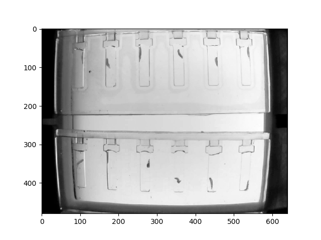
Using this option corrects this artifact using openCV functions. An in-depth explanation can be found on their website.
After running the algorithm on the image shown above, the lines appear significantly straighter now:
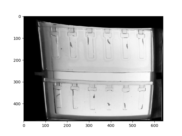
Important
The algorithm needs two matrices, dist.npy and mtx.npy which are provided for the standard Raspberry Pi camera lens. If you are using a different lens, you must redefine these matrices. Please see here or here to learn how to update them.
There are several options available to define the desired output:
avi/mp4/None: If you want to watch the video, it is probably a good idea to convert the video either into avi or mp4 as your video player will be better able to handle these formats (and the metadata of this file will be correct, see above). If “None” is chosen, the video will not be converted.
h264/raw video: Besides the format, the codec can be a problem for some programs you want to open a video. Here, you can choose between the efficient h264 codec which will lead to very small file sizes and the raw video codec. The latter will lead to significantly larger video files! h264 is recommended!
Save *.npy: If this checkbox is marked, the video will save each frame in a Numpy array. This can be very handy if you want to use python to run the downstream analysis of the data.
Note
Video encoding has been perfected over the years. Decompressing a video often leads to surprisingly large files, especially for long videos, or videos with a high framerate. If the uncompressed video is larger than your computer has RAM this script will most likely fail.
Save *.mat: If this checkbox is marked, the script will save the images in a Matlab like array. This can be very handy if you want to use Matlab to run downstream analysis of the data.
Note
Video encoding has been perfected over the years. Decompressing a video often leads to surprisingly large files, especially for long videos, or videos with a high framerate. If the uncompressed video is larger than your computer has RAM this script will most likely fail.
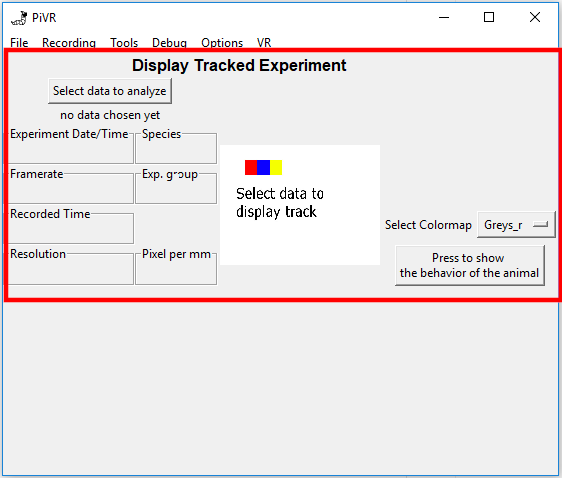
7.4. Display tracked experiment
This tool allows you to display the tracked animal in its arena similar to a video player.
The experiment must have been generated using PiVR: either on on the Raspberry Pi using the Tracking or Virtual reality or by using the post-hoc analysis option in the ‘Tools’ Menu.
Besides enabling you to conveniently see where the animal was in each frame, this tool allows you to:
Correct false Head/Tail assignments by swapping them
Save a video (in mp4 format) of the experiment.
To display an experiment, press on the “Select data to analyze” button and select a folder containing a single experiment.

The software will automatically read the metadata of the experiment and will be displayed on the left side of the GUI.
In the center, the ‘Overview of tracking.png’ file is shown.
On the right you may choose a colormap before pressing “Press to show behavior of the animal”.
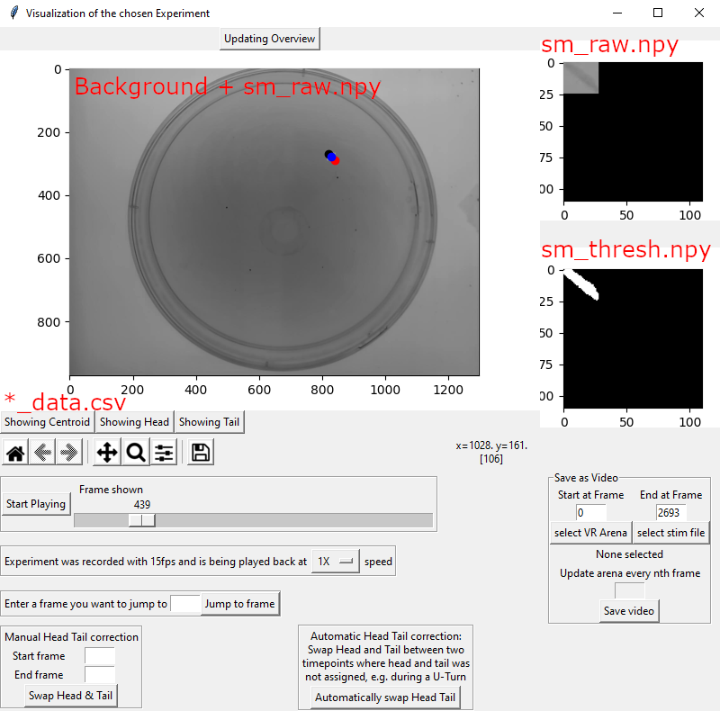
The window above will emerge as a popup. While it is open the main GUI is unavailable!
This window has the following functionality:
Updating Overview: This button will allow you to turn the main window off when playing back the experiment. This can be useful if you are only interested in the small images on the right.
The main figure in the center of the window is created by placing the raw small image (sm_raw.npy) into the reconstructed background image (Background.jpg) using the bounding box coordinates (bounding_boxes.npy). It also displays the detected Centroid, Tail and Head (*_data.csv) directly on the animal.
The three buttons below the main window on the left, “Showing Centroid”, “Showing Head” and “Showing Tail” allow you to turn off the different parts shown in the main figure.
The toolbar below allows you to interact with the main window (zoom etc.).
The slider below lets you scroll through the experiment. Pressing the “Start Playing” button will display the experiment.
The Dropdown menu below the slider lets you play back the experiment at a variety of speeds you can choose from.
If there is a particular frame you want to go to, you can enter that number in the field below and press “Jump to frame”.
If the head/tail assignment has been made incorrectly, you have two options to fix it here.
Manual Head Tail correction: Define the timepoints in which the head and tail have been incorrectly identified in ‘Start frame’ and ‘End frame. Press ‘Swap Head & Tail’
Automatic Head Tail correction: You need to slide the slider to a frame with incorrect head tail classification. Then press ‘Automatically swap Head Tail’. The algorithm will swap head and tail for previous and following frames until it finds a frame where the head and tail could not be assigned, for example during a U-Turn.
On the top right, the small raw image (sm_raw.npy) is being displayed.
Below, the binary small image (sm_thresh.npy) is being displayed.
7.4.1. Creation of a video file
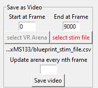
In the “Save as Video” box at the bottom right you may create a video of the experiment. There are several options to customize the output file:
Note
If you get an error message it is possible that you have not installed the correct version of ffmpeg. Usually the error message should indicate what you have to install. If you need help, please open a ticket.
If you want to create a video displaying the the animal at the correct position, all you need to do is define the start and end frame of the video and hit ‘Save Video’. If you do not want the head, tail and/or centroid to be displayed in the video, turn it off as you would for the interactive visualization.
If you have been stimulating your animal with a time dependent stimulus and you want your video to indicate when the stimulus was turned on, press the button titled ‘select stim file’ and select your stimulus file. The stimulus file must adhere to the PiVR guidlines. Then hit ‘Save Video’
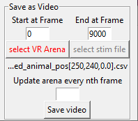
If you have been stimulating your animal with a static Virtual Arena and you want your video to indicate where the animal was relative to the position of the Virtual Arena. Press the button titled ‘select VR arena’ and select your VR file. Then hit ‘Save Video’
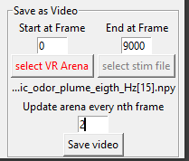
If you have been presenting your animal with a dynamic virtual reality (i.e. one that changes over time) you may also include this in the video. Press the button titled ‘select VR arena’ and select the file you used when presenting the animal with the dynamic virtual reality. Finally, indicate in ‘Update arena every nth frame’ after how many frames the arena needs to be updated. For example, if you have been presenting an arena that updates at 15Hz while recording at 30Hz you need to update every 2nd frame (30/15=2).
When pressing “Save video” the video will be saved as “Exported_Video_0.mp4” in (or “Exported_Video_1.mp4” if this is the second video that is being exported etc.) the experimental folder. This usually takes a significant amount of time, even on a fast computer.
7.5. Multi-Animal Tracking
This tool allows you to identify more than one animal in a video or in a series of images.
The identification of the animals is achieved via background subtraction of the mean image. Each animal is given an arbitrary number. In the next frame, the animal closest to that number in the previous frame is assigned.
This guide is intended to get you started quickly. If you are
interested in the more technical aspects, please see
multi_animal_tracking.MultiAnimalTracking
Note
Identifying more than one animal in an experiment is computationally challenging. There are several specialized tools such as the multiworm tracker, Ctrax, idtracker, idtracker.ai and MARGO. The PiVR multi-animal tracking software has not been benchmarked against these tools. This software has several limitations. It is probably ok to use in cases where you are interested in counting how many animals are in a general area. It is not recommend to use the tracker for other parameters, such as calculating animal speed (due to loss of identity after collision and ‘jumps’ in the trajectory) and similar parameters.
After selecting a folder containing a video of image sequence of an experiment containing multiple animals, press the “Press to show the behavior of the animals” button.
The software will now load the image data (which can take a considerable amount of time) and display a new window which will help you to optimize the tracking parameters.
Note
You might notice that the image is distorted. This is due to the Raspberry Pi camera lens. See here.
First, have a look at the all-important “# of animals in the current frame” on the bottom right of the popup. In this video there are only 6 animals, but the algorithm detects 10 objects as “animals”. The blobs identified as animals are indicated using small rectangles in the main figure.
Important
The goal is to have have as many frames as possible contain only the expected amount of animals.
To achieve this goal, start by defining the area in which animals can move into. In this particular experiment, the outline of the petri dish can be clearly seen:
Press the “Select Rectangular ROI”. The button will turn red.
Using the mouse, create a rectangle in the main window. The result is indicated. The “# of animals in the current frame” is immediately updated.
While this is already better, there are still two blobs wrongly identified as animals, one at (y=300,x=100) and the other at (y=270, x=480).
By increasing the “Threshold (STD from Mean) number these mis-identified blobs are not mistaken for animals animal:
There are now no mis-identified animals. While there are a total of 6 animals in the image, the algorithm can only detect 5. To understand why that is the case, press the magnifying class symbol below the main figure and draw a rectangle around the region you want to enlarge.
It is now obvious that 4 out of 6 animals are properly identified. Two of the animals, at (y=260, x=360) are very close to each other and are identified as one animals, however. There is no way for this tracking algorithm to separate animals that are touching each other!
Now you need to make sure that the image parameters are such that you get the expected animal number in all frames. To not have to go through each of the frames manually, you can just press “Auto-detect blobs” on the bottom right. This will run a script that will take the current image detection parameters into account and just count how many blobs are counted as animals. The result is plotted in the figure on the top right.
This result indicates that at the beginning of the video there are several frames where only 5 animals can be detected. By visually inspecting these frames it becomes obvious that this is due to the two animals touching each other as they already do in the first frame.
Next, find frames that have the wrong amount of animals. Try to fix them using the image parameter settings.
There can be situations where the animal number will just be wrong and it can not be fixed. The algorithm can handle this if the number of those frames is low.
Once you have optimized the image parameters, go to the frame where the correct amount of animals is detected. This is crucial as it tell the algorithm how many animals to expect!. Then press “Track animals”.
A new popup will open. It indicates how many animals (and where) are detected in this frame. Each animal gets an arbitrary number. If the number of animals is correct, press “Looks good, start tracking”. Else press “Not good, take me back”.
The tracking itself is computationally quite expensive and therefore usually takes a while to complete. To speed up tracking, you can press the “Updating Overview” button above the main window.
Once tracking has concluded the result will be displayed in the main window as shown below.
If there are huge gaps in the trajectory, for example because an animal could not be detected for a while, you can press the “interpolate centroids” button. This will calculate realistic possible distances travelled (based on ‘Max Speed Animal[mm/s]) between frames and try to connect trajectories. This is a untested feature - use at your own risk. Ideally you should not have to use this option.
7.5.1. Multi Animal Tracking Output
After using the Multi-Animal Tracker, you will find two new files in the experimental folder:
The “Background.npy” file which is just the mean of all images, resulting in the background image used during tracking.
The “XY_positions.csv” file contains the X and Y coordinates for each identified animal for each frame. For frames with not enough animals, the corresponding row will be empty.
7.6. Creating a new Virtual Arena
How to create a new virtual arena, the essential tool that gives PiVR its name?
First, a brief overview of what the different elements of an arena file mean:
You can find several example virtual arena files in the PiVR/VR_arenas folder: As an example lets analyze “640x480_checkerboard.csv”
The file itself is a 2D matrix with 640 columns and 480 rows. Each value in the matrix defines what happens on that pixel on the camera.
For example, if you define the value 100 at position column = 75 and row = 90 here in the virtual arena and then present this virtual arena to the animal using the Closed Loop stimulation tab on PiVR, if the animal is at pixel column = 75 and row = 90 the intensity of 100 will be played back.
A big advantage of virtual realities over real environments is the control the experimenter has over the experimental conditions. When running an experiment, one often has to repeat trials many times. In real environments, the experimenter can never have identical initial conditions, e.g. the animals is placed at a slightly different position, the animal moves in different conditions before the tracking even starts etc. With virtual reality, this factor (which often introduces variability into data) can be alleviated. The experimenter can define a virtual reality arena and the animal will always be presented with the identical initial conditions.
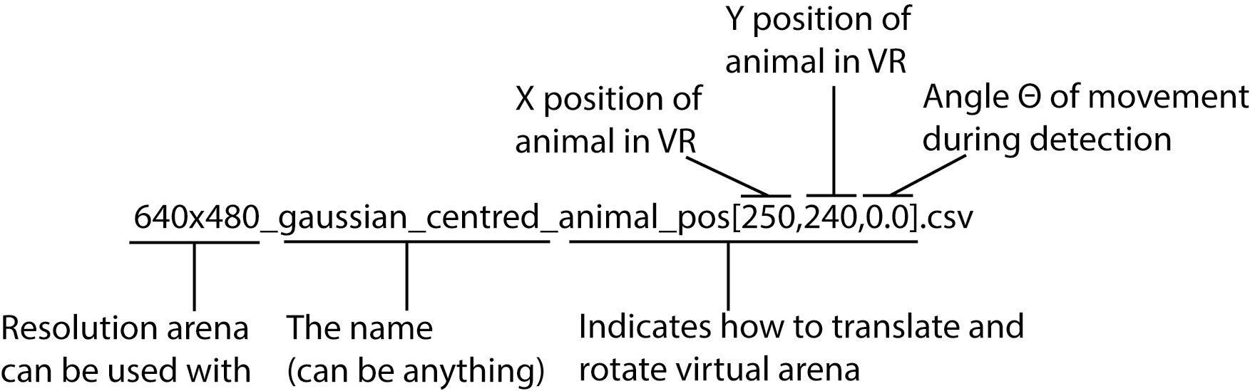
To do this, lets examine another example virtual arena file you can find in PiVR/VR_arenas: “640x480_gaussian_centred_animal_pos[250, 240,0.0].csv”
This file has a string at the end of its filename: animal_pos[250, 240,0.0]. This string indicates where the animal must start in relation to the virtual reality. In this example, wherever the animal is in the real image when the experiment starts, the virtual reality will be translated so that it is at x-coordinate 250 and y coordinate 240.
In addition, if the third value (here 0.0) is defined, the movement of the animal during detection is taken into account: The virtual arena is rotated so that the animal always starts going into the same direction relative to the virtual arena. The angle you may use goes from -pi to +pi (see atan2).
If you want to create a virtual reality arena from scratch, for example in python, all you need to do is create a matrix with the correct dimension, fill it with values between 0 and 100 as you see fit and export the file as csv.
import numpy as np

virtual_arena = np.zeros((480,640),dtype=np.float64)
# Define parts of the arena where the animal is supposed to be
# stimulated e.g. by typing
virtual_arena[:,0:100] = 100
virtual_arena[:,101:200] = 75
virtual_arena[:,201:300] = 50
# this will give you a very coarse grained virtual arena that will
# stimulate strongly if the animal is on the left side, stimulate
# 75% if the animal is a bit more on the right and 50% if it is
# still on the left but almost in the middle. The rest is
# unstimulated as of yet.

# Now you need to save the arena. Let say you want to have the animal
# start ascending the gradient from the middle (essentially animal
# has to move to the left in the virtual arena)
np.savetext("Path/On/Your/PC/640x480_my_awesome_arena_animal_pos[300,240,0.0].csv")
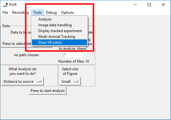
Alternatively, you can use the “Tools->Draw VR Arena” option on the PC version of PiVR.
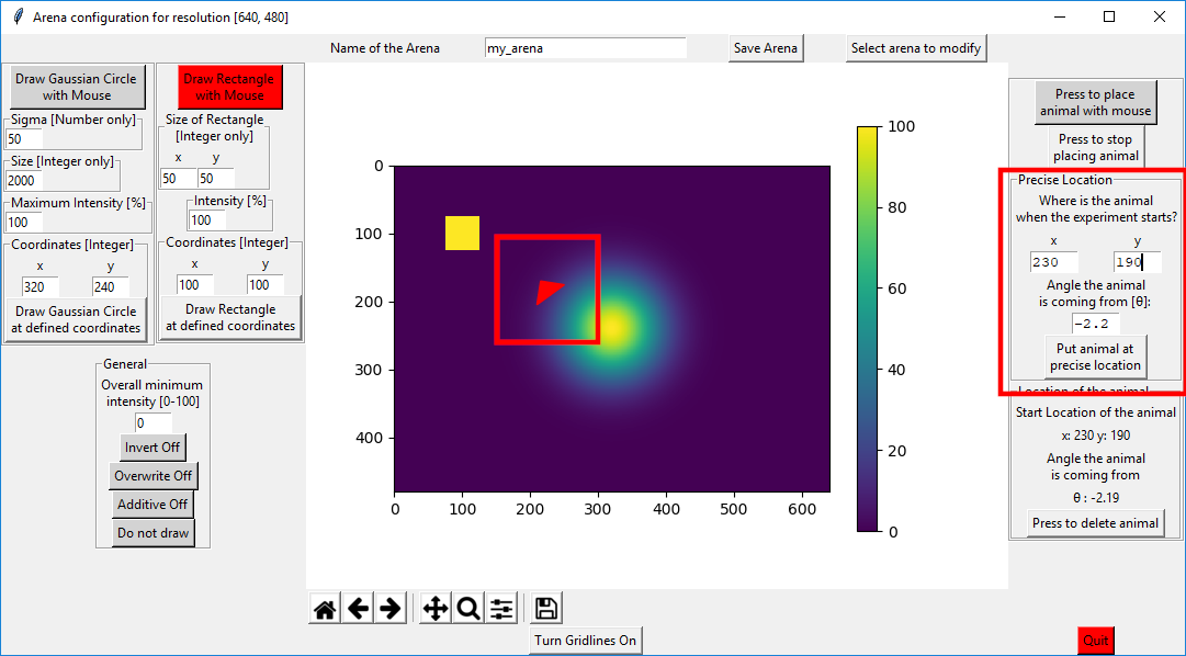
You will find the following empty canvas. You can open a previously defined virtual arena or work on the blank canvas. Either way, you have the the option to create gaussian shaped 2D circles and rectangles. To “draw” such a gaussian shaped 2D circle, you can either press on “Draw Gaussian Circle with Mouse” (and then click somewhere on the canvas) or you can press on “Draw Gaussian Circle at defined coordinates”.
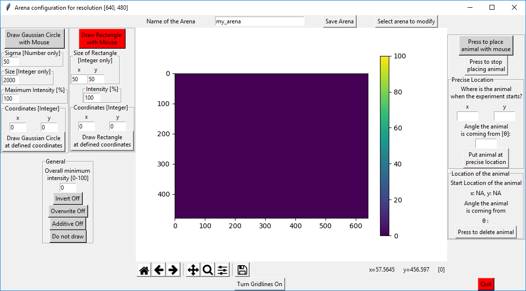
You can change the Gaussian shaped 2D circle by changing its Sigma, its size and the intensity.
Analogous, you can define the size and the intensity of the rectangle by entering the desired value.
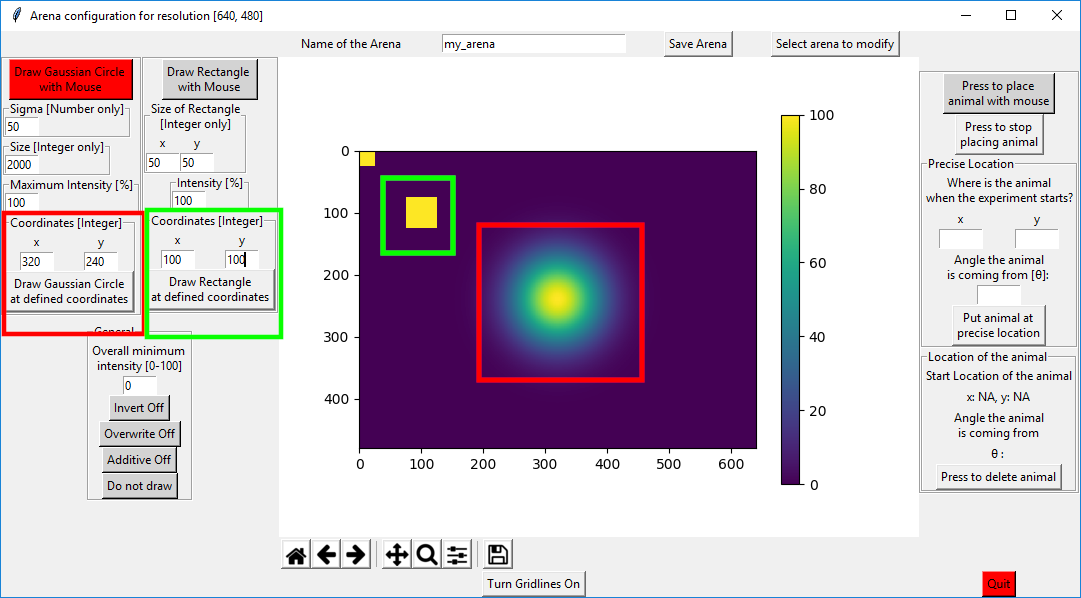
In the example below, I used the standard settings for the gaussian circle size but changed the “Coordinates” to the values shown. Then I pressed on “Draw Gaussian Circle at defined coordinates”(red squares). Then I modified the “Coordinates” of the rectangle on the right to x=100 and y=100 and pressed on “Draw Rectangle at defined coordinates” (green squares).
There are 3 additional buttons that expand the possibilities of drawing virtual arenas:
Invert: If this is on, whenever you draw a circle or rectangle, it subtracts the values from the intensity that is already present. This option was used to create the following virtual arena: “640x480_volcano_animal_pos[320,240,0.0].csv”
Overwrite: will just overwrite the previous pixel values with the new values with no regard to the previous value (as opposed to “Invert” and “Additive”)
Additive: If you place a 50% rectangle somewhere and then place another on top of it, usually nothing will happen as the absolute value is being drawn. If this is on, the values are “added”.
Note
If you go above 100%, everything will be normalized.
On the right side of the canvas you can define the starting position of the animal in the virtual arena. Besides just x and y position, you can define the direction from which the animal is coming from.
You can use the mouse, either by clicking (just x and y position) or by clicking and dragging (x, y and angle). Alternatively, you can use precise coordinates.
Note
Angle can go from -pi to +pi. See atan2 for visualization.
Once you are done with the arena, make sure to save it. Then you can just quit the window.
7.7. Creating a new Dynamic Virtual Reality
Before attempting to create a new dynamic virtual reality please make sure you understand exactly how a static virtual reality is created.
The main differences between the static and the virtual reality are:
Usage of numpy arrays instead of csv files.
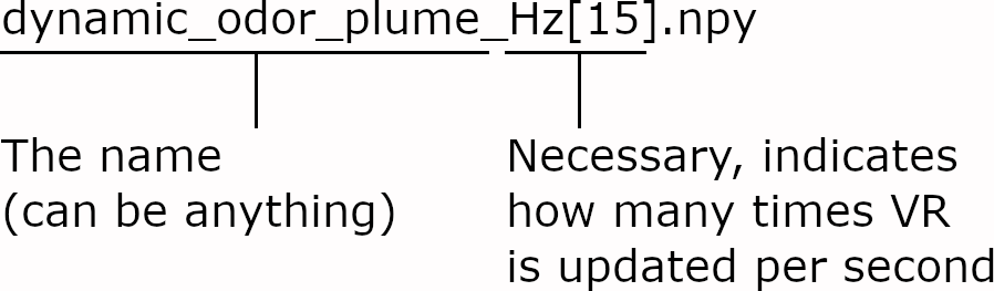
The filename includes the speed at which the virtual reality is “played back” as a “Hz[#]” term.
Instead of going from 0 - 100, stimulation in defined as 8 bit (0 - 255)
For details on how exactly this is implemented, please see here
There are several limitations compared to static virtual realities:
Dynamic virtual realities can not orient themselves relative to the the position of the animal at the start of the experiment.
RAM of PiVR is limited (but this is getting better with the RPi4 which has up to 4Gb). As the arena that is presented must be loaded into RAM at the beginning of the experiment, it can not be too large. On our RPi3+ (1Gb of RAM) we successfully used dynamic virtual realities of 135Mb for 5 minute experiments.
It is not possible to use the “Adjust Power” field!
How does a dynamic virtual reality file look like? Essentially it is just the 3D version of the static virtual arena with the difference that an integer value of 255 indicates that the LED is completely on (as opposed to 100 in the static case). The third axis contains all the ‘frames’ of the virtual reality ‘video’.
As an example, follow the instructions below to convert a real odor plume measurement to a dynamic virtual reality that PiVR can use:
Get the odor plume data from Álvarez-Salvado et al ., 2018 and unzip the file. The relevant file is “10302017_10cms_bounded_2.h5”.
While downloading, you can make sure you have the correct conda environment to handle the data. Below is the code to create new environment and install the necessary packages (Windows):
conda create -n dynamic_odor_env python=3.7 -y
activate dynamic_odor_env
conda install -c anaconda h5py -y
conda install matplotlib -y
Now start python and adapt the following code:
import numpy as np
import h5py

# Adapt this to the location of your file
data_path = 'C:\\10302017_10cms_bounded_2.h5'

# Read the h5 datafile using the h5py library
data = h5py.File(data_path, 'r')

# The h5 datafile is a dictionary. As the keys are unkown,
# cycle through to learn what files are stored in this fie.
for key in data.keys():
   print(key) #Names of the groups in HDF5 file.
# ok, the relevant (only) key is 'dataset2'
# Using this group key we can now access the data
actual_data_temp = data['dataset2']
actual_data = actual_data[()]
# make sure you do have the data:
print(actual_data.shape)
# (3600, 406, 216)
# This information, together with the metadate indicates that
# the first dimension holds the measurements of the timepoints
# (Frequency of 15Hz for a duration of 4 minutes = 3600 frames).
# The other two dimensions are spatial dimensions.

# Below the reason it is necessary to use uint8 (8bit integer
# precision instead of float (just remove the #)
# import sys
# print('Using 64bit float precision: ' +
#    repr(sys.getsizeof(np.zeros((actual_data.shape[0],640,480),
#    dtype=np.float64))/1e6) + 'Megabytes' )
# print('Better to use uint8 as I ll only need to use: ' +
#    repr(sys.getsizeof(np.zeros((actual_data.shape[0],640, 480),
#    dtype=np.uint8))/1e6) + 'Megabytes in RAM' )

# Now to convert the 64bit floating point to 8 bit
# find maximum value:
max_value = np.amax(actual_data)
# find minimum value:
min_value = np.amin(actual_data)

# convert data to uint8 to save a ton of space
convert_factor = 255/(max_value + (- min_value))
downsampled = (actual_data+(-min_value)) * convert_factor

 # We need to create an empty arena with 640x480 pixels using the
 # correct datatype..
 correct_size_arena = np.zeros((480,640,actual_data.shape[0]),
    dtype=np.uint8)
 # and place the moving arena in to the center.
 start_y = int(correct_size_arena.shape[0]/2 -
    downsampled.T.shape[0]/2) # 132.0
 start_x = int((correct_size_arena.shape[1]/2 -
     downsampled.T.shape[1]/2)) # 117
 correct_size_arena[start_y:int(start_y+downsampled.T.shape[0]),
    start_x:int(start_x+downsampled.T.shape[1]),:] = downsampled.T

 # In order to see how the just created arena looks like, run
 # the code below (uncomment by removeing the #)
 # import matplotlib.pyplot as plt
 # fig,ax = plt.subplots()
 # ax.imshow(correct_size_arena[:, :, 0])
 # plt.show()

 # Even after downsampling, file is way to large (>1Gb). To
 # solve this, only save 1/8 of the file (~30seconds).
 np.save('C:\\dynamic_odor_plume_eigth_Hz[15].npy',
    correct_size_arena[:,:,0:int(correct_size_arena.shape[2]/8)])
Now you must transfer the file containing the new dynamic virtual reality to your PiVR setup and select it when running your experiment, identical to what you would do to select a static virtual arena.