PiVR has been developed by David Tadres and Matthieu Louis (Louis Lab).
6. Explanation of PiVR output
6.1. Tracking
After running a tracking experiment you will find a folder with the “DATE_TIME_EXP.GROUP” as its name. An example would be “2019.01.11_14-00-05_CantonS”. This is an experiment conducted on the 11th of January 2019. “CantonS” is the value that was entered in the field “Exp. Group”.
This folder will contain the following files:
6.1.1. “DATE_TIME_data.csv”
is probably the most important file. It contains the following data for each frame of the experiment:
The frame (=image) number into the experiment
The time in seconds since the experiment started
The X (column) coordinate of the Centroid (Check here for comparison with midpoint)
The Y (row) coordinate of the Centroid
The X (column) coordinate of the head
The Y (row) coordinate of the head
The X (column) coordinate of the tail
The Y (row) coordinate of the tail
The X (column) coordinate of the midpoint (Check here for comparison with centroid)
The Y (row) coordinate of the midpoint
The Y-min (row) coordinate of the bounding box (See here for explanation
The Y-max (row) coordinate of the bounding box.
The X-min (row) coordinate of the bounding box.
The X-max (row) coordinate of the bounding box.
The local threshold used to extract the binary image during tracking.
6.1.2. “Background.jpg”
contains the reconstructed background image. See here for explanation where it is coming from and what it means.
6.1.3. “experiment_settings.json”
is a json file and contains a lot of useful experimental information:
Camera Shutter Speed [us]: Shutter speed in microseconds
Exp. Group: The string that was entered by the user during the experiment
Experiment Date and Time: exactly that
Framerate: The frequency at which PiVR tracked the animal
Model Organism: While tracking, PiVR used the parameters of this animal to optimize tracking. See here for how to modify this parameter.
PiVR info (recording): version number, git branch and git hash of the PiVR software that was used to record the experiment.
PiVR info (tracking): version number, git branch and git hash of the PiVR software that was used to track the experiment. If online tracking is being done, this is identical to the info above.
Pixel per mm: For PiVR to be able to track the animal, it needs to know how many pixels indicate one mm. This has been set by the user as described here.
Recording time: The time in seconds that PiVR was tracking the animal
Resolution: The camera resolution in pixels that PiVR used while tracking.
Time delay due to Animal Detection[s]: For the autodetection the animal must move. The time it took between pressing “start” and successful animal detection is saved here.
Virtual Reality arena name: If no virtual arena was presented, it will say ‘None’
backlight 2 channel: If Backlight 2 has been defined (as described here) the chosen GPIO (e.g. 18) and the maximal PWM frequency (e.g. 40000) is saved as a [list].
backlight channel: If Backlight 1 has been defined (as described here) the chosen GPIO (e.g. 18) and the maximal PWM frequency (e.g. 40000) is saved as a [list]. This would normally be defined as [18, 40000].
output channel 1: If Channel 1 has been defined (as described here) the chosen GPIO (e.g. 17) and the maximal PWM frequency (e.g. 40000) is saved as a [list].
output channel 2: If Channel 2 has been defined (as described here) the chosen GPIO (e.g. 27) and the maximal PWM frequency (e.g. 40000) is saved as a [list].
output channel 3: If Channel 3 has been defined (as described here) the chosen GPIO (e.g. 13) and the maximal PWM frequency (e.g. 40000) is saved as a [list].
output channel 4: If Channel 4 has been defined (as described here) the chosen GPIO (e.g. 13) and the maximal PWM frequency (e.g. 40000) is saved as a [list].
Setup Name: The name of the setup if entered by user (see here). If nothing has been entered by user it will read ‘myPiVR-init_DATE’ with DATE indicating the date the Raspberry Pi showed when the PiVR software was first opened.
6.1.4. “first_frame_data.json”
is a json file and contains
information that collected during
animal detection (Source
code pre_experiment.FindAnimal.)
bounding box col max: The X_max value of the bounding box of the animal detected in the first frame during animal detection.
bounding box col min: The X_min value of the bounding box of the animal detected in the first frame during animal detection.
bounding box row max: The Y_min value of the bounding box of the animal detected in the first frame during animal detection.
bounding box row min: The Y_max value of the bounding box of the animal detected in the first frame during animal detection.
centroid col: The X value of the centroid of the animal detected in the first frame during animal detection.
centroid row: The Y value of the centroid of the animal detected in the first frame during animal detection.
filled area: The filled area in pixels of the blob defined as the animal in the first frame during animal detection
6.1.5. “sm_raw.npy”
is a Numpy file. It contains the small image.
This file comes in shape [“y size”, “x size”, # of frames]. “y size” == “x size” and is defined based on the organism and px/mm. Specifically, it is 2*’max_skeleton_length_mm’ * pixel_per_mm to ensure the animal fits into the array.
6.1.6. “sm_thresh.npy”
is a Numpy file. It contains the binarized small image.
This file comes in shape [“y size”, “x size”, # of frames]. “y size” == “x size” and is defined based on the organism and px/mm. Specifically, it is 2*’max_skeleton_length_mm’ * pixel_per_mm to ensure the animal fits into the array.
6.1.7. “sm_skeletons.npy”
is a Numpy file. It contains the skeleton of the tracked animal.
This file comes in shape [“y size”, “x size”, # of frames]. “y size” == “x size” and is defined based on the organism and px/mm. Specifically, it is 2*’max_skeleton_length_mm’ * pixel_per_mm to ensure the animal fits into the array.
6.1.8. “undistort_matrices.npz”
contains the undistort files used to correct for lens distortion of the image.
The file contains two objects, ‘mtx’ and ‘dist’ which are used by the cv2.undistortPoints function.
6.1.9. Optional files
The rest of this subsection describes files that need to be explicitly saved as described here.
6.1.9.1. “bounding_boxes.npy”
is a Numpy file. It contains the coordinates of the bounding box of the small image. The bounding box defines the Y/X coordinates of the small image.
This file comes in shape [4, # of frames] with:
[0, :] |
contains the Y_min values |
[1, :] |
contains the Y_max values |
[2, :] |
contains the X_min values |
[3, :] |
contains the X_max values |
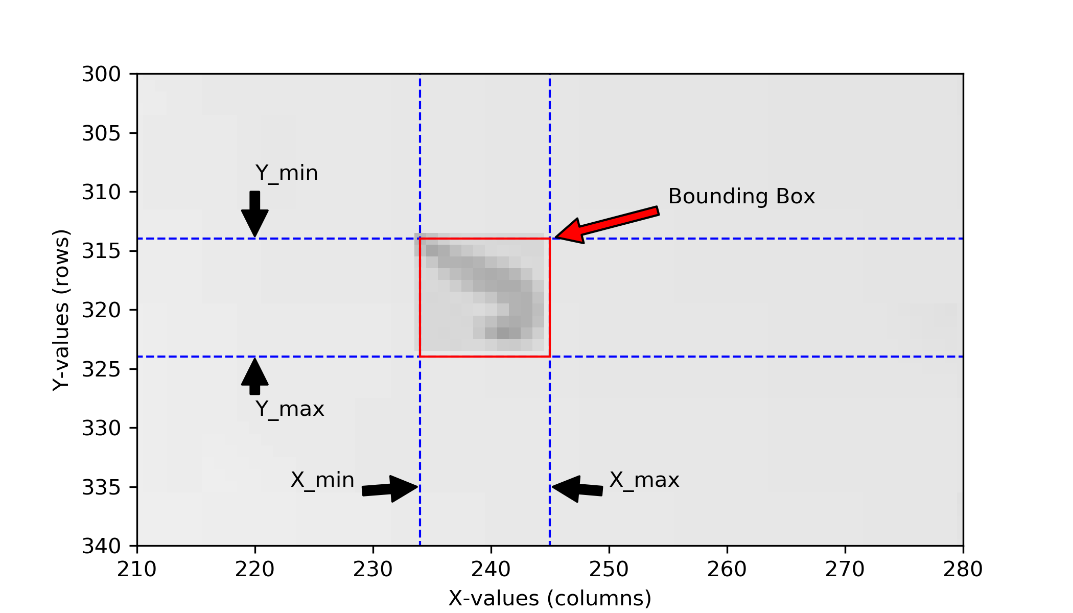
These values are necessary to describe where in the full image frame the small image that has been saved during the experiment is located. The bounding box is the rectangle that contains all image information used during this frame. Below an illustration on how the different values are used to construct the bounding box.
Note
Why Y/X and not X/Y? In image processing the convention is to reference points in (Rows, Columns) which translates to Y/X. The underlying image processing libraries work with the (Rows, Columns) convention. See for example here. PiVR therefore follows this convention.
6.1.9.2. “centroids.npy”
is a Numpy file. It contains the coordinates of the centroid of the blob identified during the experiment. See here to see the centroid compared to the midpoint.
The file comes in shape [# of frames, 2] with:
[:, 0] |
contains the centroid Y values |
[:, 1] |
contains the centroid X values |
These values are identical to what you will find in the “DATE_TIME_data.csv” file
6.1.9.3. “midpoints.npy”
is a Numpy file. It contains the coordinates of the midpoint extracted from the skeleton during the experiment. See here to see the midpoint compared to the centroid.
The file comes in shape [# of frames, 2] with:
[:, 0] |
contains the midpoint Y values |
[:, 1] |
contains the midpoint X values |
These values are identical to what you will find in the “DATE_TIME_data.csv” file
6.1.9.4. “heads.npy”
is a Numpy file. It contains the coordinates of the head position assigned during tracking.
The file comes in shape [# of frames, 2] with:
[:, 0] |
contains the head Y values |
[:, 1] |
contains the head X values |
These values are identical to what you will find in the “DATE_TIME_data.csv” file
6.1.9.5. “tails.npy”
is a Numpy file. It contains the coordinates of the tail position assigned during tracking.
The file comes in shape [# of frames, 2] with:
[:, 0] |
contains the tail Y values |
[:, 1] |
contains the tail X values |
These values are identical to what you will find in the “DATE_TIME_data.csv” file
6.2. VR Arena and Dynamic VR Arena
After running a VR Arena experiment you will find a folder with the “DATE_TIME_EXP.GROUP” as its name. An example would be “2019.01.11_14-00-05_CantonS”. This is an experiment conducted on the 11th of January 2019. “CantonS” is the value that was entered in the field “Exp. Group”.
This folder will contain the following files:
6.2.1. “DATE_TIME_data.csv”
is probably the most important file. It contains the following data for each frame of the experiment:
The frame (=image) number into the experiment
The time since the experiment started
The X (column) coordinate of the Centroid (Check here for comparison with midpoint)
The Y (row) coordinate of the Centroid
The X (column) coordinate of the head
The Y (row) coordinate of the head
The X (column) coordinate of the tail
The Y (row) coordinate of the tail
The X (column) coordinate of the midpoint (Check here for comparison with centroid)
The Y (row) coordinate of the midpoint
The Y (row) coordinate of the midpoint
The Y-min (row) coordinate of the bounding box (See here for explanation
The Y-max (row) coordinate of the bounding box.
The X-min (row) coordinate of the bounding box.
The X-max (row) coordinate of the bounding box.
The local threshold used to extract the binary image during tracking.
The stimulus delivered stimulus in %
6.2.2. “RESOLUTION_NAME.csv”
for example “640x480_checkerboard.csv”. This is the virtual arena presented to the animal. In case the virtual arena is positioned relative to the starting position and the movement of the animal (such as the “640x480_gaussian_centred_animal_pos[250,240,0.0].csv” arena), this file will final translated and rotated arena as it was presented to the animal.
Note
If a dynamic virtual reality has been presented, this file will not be present - it would simply take too long and take up too much space. This is one reason why dynamic virtual realities can not be translated and rotated at the moment.
6.2.3. “Background.jpg”
contains the reconstructed background image. See here for explanation where it is coming from and what it means.
6.2.4. “experiment_settings.json”
is a json file and contains a lot of useful experimental information:
Search box size: The Search box used to locate the animal during the experiment
Exp. Group: The string that was entered by the user during the experiment
Experiment Date and Time: exactly that
Framerate: The frequency at which PiVR tracked the animal
Model Organism: While tracking, PiVR used the parameters of this animal to optimize tracking. See Todo here for how to modify this parameter.
Pixel per mm: For PiVR to be able to track the animal, it needs to know how many pixels indicate one mm. This has been set by the user as described here.
Recording time: The time in seconds that PiVR was tracking the animal
Resolution: The camera resolution in pixels that PiVR used while tracking.
Time delay due to Animal Detection[s]: For the autodetection the animal must move. The time it took between pressing “start” and successful animal detection is saved here.
Virtual Reality arena name: As no virtual arena was presented, it will say ‘None’
backlight 2 channel: If Backlight 2 has been defined (as described here) the chosen GPIO (e.g. 18) and the maximal PWM frequency (e.g. 40000) is saved as a [list].
backlight channel: If Backlight 1 has been defined (as described here) the chosen GPIO (e.g. 18) and the maximal PWM frequency (e.g. 40000) is saved as a [list]. This would normally be defined as [18, 40000].
output channel 1: If Channel 1 has been defined (as described here) the chosen GPIO (e.g. 17) and the maximal PWM frequency (e.g. 40000) is saved as a [list].
output channel 2: If Channel 2 has been defined (as described here) the chosen GPIO (e.g. 27) and the maximal PWM frequency (e.g. 40000) is saved as a [list].
output channel 3: If Channel 3 has been defined (as described here) the chosen GPIO (e.g. 13) and the maximal PWM frequency (e.g. 40000) is saved as a [list].
output channel 4: If Channel 4 has been defined (as described here) the chosen GPIO (e.g. 13) and the maximal PWM frequency (e.g. 40000) is saved as a [list].
Setup Name: The name of the setup if entered by user (see here). If nothing has been entered by user it will read ‘myPiVR-init_DATE’ with DATE indicating the date the Raspberry Pi showed when the PiVR software was first opened.
6.2.5. “first_frame_data.json”
is a json file and contains
information that collected during
animal detection (Source
code pre_experiment.FindAnimal.)
bounding box col max: The X_max value of the bounding box of the animal detected in the first frame during animal detection.
bounding box col min: The X_min value of the bounding box of the animal detected in the first frame during animal detection.
bounding box row max: The Y_min value of the bounding box of the animal detected in the first frame during animal detection.
bounding box row min: The Y_max value of the bounding box of the animal detected in the first frame during animal detection.
centroid col: The X value of the centroid of the animal detected in the first frame during animal detection.
centroid row: The Y value of the centroid of the animal detected in the first frame during animal detection.
filled area: The filled area in pixels of the blob defined as the animal in the first frame during animal detection
6.2.6. Optional files
The rest of this subsection describes files that need to be explicitly saved as described here. TODO LINK
6.2.6.1. “bounding_boxes.npy”
is a Numpy file. It contains the coordinates of the bounding box of the small image. The bounding box defines the Y/X coordinates of the small image
This file comes in shape [4, # of frames] with:
[0, :] |
contains the Y_min values |
[1, :] |
contains the Y_max values |
[2, :] |
contains the X_min values |
[3, :] |
contains the X_max values |
These values are necessary to describe where in the full image frame the small image that has been saved during the experiment is located. The bounding box is the rectangle that contains all image information used during this frame. Below an illustration on how the different values are used to construct the bounding box.
Note
Why Y/X and not X/Y? In image processing the convention is to reference points in (Rows, Columns) which translates to Y/X. The underlying image processing libraries work with the (Rows, Columns) convention. See for example here. PiVR therefore follows this convention.
6.2.6.2. “centroids.npy”
is a Numpy file. It contains the coordinates of the centroid of the blob identified during the experiment. See here to see the centroid compared to the midpoint.
The file comes in shape [# of frames, 2] with:
[:, 0] |
contains the centroid Y values |
[:, 1] |
contains the centroid X values |
These values are identical to what you will find in the “DATE_TIME_data.csv” file
6.2.6.3. “midpoints.npy”
is a Numpy file. It contains the coordinates of the midpoint extracted from the skeleton during the experiment. See here to see the midpoint compared to the centroid.
The file comes in shape [# of frames, 2] with:
[:, 0] |
contains the midpoint Y values |
[:, 1] |
contains the midpoint X values |
These values are identical to what you will find in the “DATE_TIME_data.csv” file
6.2.6.4. “heads.npy”
is a Numpy file. It contains the coordinates of the head position assigned during tracking.
The file comes in shape [# of frames, 2] with:
[:, 0] |
contains the head Y values |
[:, 1] |
contains the head X values |
These values are identical to what you will find in the “DATE_TIME_data.csv” file
6.2.6.5. “tails.npy”
is a Numpy file. It contains the coordinates of the tail position assigned during tracking.
The file comes in shape [# of frames, 2] with:
[:, 0] |
contains the tail Y values |
[:, 1] |
contains the tail X values |
These values are identical to what you will find in the “DATE_TIME_data.csv” file
6.2.6.6. “stimulation.npy”
is a Numpy file. It contains the stimulus delivered to the animal during the experiment.
These values are identical to what you will find in the “DATE_TIME_data.csv” file
6.3. Full Frame Recording
After taking a lot of images with Full Frame Recording, find a folder with the “DATE_TIME_EXP_GROUP” as its name. An example would be “2019.01.11_14-00-05_CantonS”. This is an experiment conducted on the 11th of January 2019. “CantonS” is the value that was entered in the field “Exp. Group”.
6.3.1. “DATE_TIME_timestamps” OR “DATE_TIME_stimulation_presented.csv”
If no time dependent stimulus has been presented, you will find a “DATE_TIME_timestamps.csv” file in the folder containing:
Frame (=image) number into the experiment
Time in seconds since the experiment started
If a time dependent stimulus was presented, you will find a “DATE_TIME_stimulation_presented.csv” file in the folder containing:
Frame (=image) number into the experiment
Time in seconds since the experiment started
Channel 1 stimulus delivered
Channel 2 stimulus delivered
Channel 3 stimulus delivered
Channel 4 stimulus delivered
6.3.2. Image files
Usually lots upon lots of them. Each image is saved separately directly into this folder.
6.3.3. “experiment_settings.json”
is a json file and contains a lot of useful experimental information:
Experiment Date and Time: Exactly as advertised
Framerate: The framerate the video was recorded in
Exp. Group: The string that was entered by the user during the experiment
Model Organism: If selected, what animal has been indicated during the experiment.
Pixel per mm: If defined (see here) a useful parameter for analysis.
Recording time: The time in seconds that PiVR was recording this video.
Resolution: The camera resolution in pixels that PiVR used while recording the video.
Virtual Reality arena name: As no virtual arena was presented, it will say ‘None’
backlight 2 channel: If Backlight 2 has been defined (as described here) the chosen GPIO (e.g. 18) and the maximal PWM frequency (e.g. 40000) is saved as a [list].
backlight channel: If Backlight 1 has been defined (as described here) the chosen GPIO (e.g. 18) and the maximal PWM frequency (e.g. 40000) is saved as a [list]. This would normally be defined as [18, 40000].
output channel 1: If Channel 1 has been defined (as described here) the chosen GPIO (e.g. 17) and the maximal PWM frequency (e.g. 40000) is saved as a [list].
output channel 2: If Channel 2 has been defined (as described here) the chosen GPIO (e.g. 27) and the maximal PWM frequency (e.g. 40000) is saved as a [list].
output channel 3: If Channel 3 has been defined (as described here) the chosen GPIO (e.g. 13) and the maximal PWM frequency (e.g. 40000) is saved as a [list].
output channel 4: If Channel 4 has been defined (as described here) the chosen GPIO (e.g. 13) and the maximal PWM frequency (e.g. 40000) is saved as a [list].
Setup Name: The name of the setup if entered by user (see here). If nothing has been entered by user it will read ‘myPiVR-init_DATE’ with DATE indicating the date the Raspberry Pi showed when the PiVR software was first opened.
6.3.4. (Optional) stimulation_file_used.csv
If a time dependent stimulus was presented, the original stimulus file is saved in the experimental folder.
6.4. Video
After recording a video, you will find a folder with the “DATE_TIME_EXP.GROUP” as its name. An example would be “2019.01.11_14-00-05_CantonS”. This is an experiment conducted on the 11th of January 2019. “CantonS” is the value that was entered in the field “Exp. Group”.
6.4.1. “EXPGRP_VIDEO.h264”
is the video file. This video file on its own is not perfectly useful (at least in my hands) as h264 seems to be a bit of an exotic file format that many video players can not handle without problems.
In order to directly convert this file, see the Image Data handling instructions. If you want to a GUI-free version of these modules, check out the “convert_h264_to_AVI.py” at https://gitlab.com/davidtadres/pivr_bonus
Note
I have tried to directly convert the image using ffmpeg. I believe there is a bug somewhere in the encoder of the camera as ffmpeg reads that the video is “inf” long. The scripts above take the video metadata from “experiment_settings.json” to properly convert the video.
The standard lens introduces a lot of radial aberrations at the edges! To fix them see undistort h264 video.
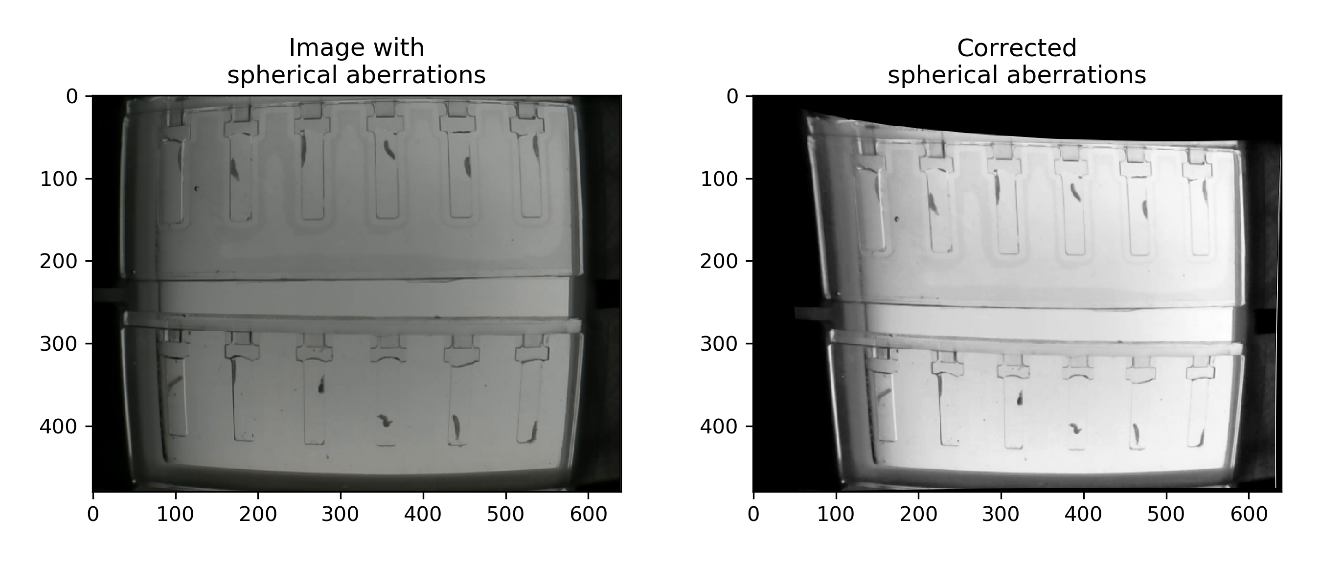
To correct these distortions, just make sure you have selected Perform Undistort before running the video conversion.
6.4.2. “DATE_TIME_timestamps” OR “DATE_TIME_stimulation_presented.csv”
If no time dependent stimulus has been presented, you will find a “DATE_TIME_timestamps.csv” file in the folder containing:
Frame (=image) number into the experiment
Time in seconds since the experiment started
If a time dependent stimulus was presented, you will find a “DATE_TIME_stimulation_presented.csv” file in the folder containing:
Frame (=image) number into the experiment
Time in seconds since the experiment started
Channel 1 stimulus delivered
Channel 2 stimulus delivered
Channel 3 stimulus delivered
Channel 4 stimulus delivered
6.4.3. “experiment_settings.json”
is a json file and contains a lot of useful experimental information:
Experiment Date and Time: Exactly as advertised
Framerate: The framerate the video was recorded in
Exp. Group: The string that was entered by the user during the experiment
Model Organism: If selected, what animal has been indicated during the experiment.
Pixel per mm: If defined (see here) a useful parameter for analysis.
Recording time: The time in seconds that PiVR was recording this video.
Resolution: The camera resolution in pixels that PiVR used while recording the video.
Virtual Reality arena name: As no virtual arena was presented, it will say ‘None’
backlight 2 channel: If Backlight 2 has been defined (as described here) the chosen GPIO (e.g. 18) and the maximal PWM frequency (e.g. 40000) is saved as a [list].
backlight channel: If Backlight 1 has been defined (as described here) the chosen GPIO (e.g. 18) and the maximal PWM frequency (e.g. 40000) is saved as a [list]. This would normally be defined as [18, 40000].
output channel 1: If Channel 1 has been defined (as described here) the chosen GPIO (e.g. 17) and the maximal PWM frequency (e.g. 40000) is saved as a [list].
output channel 2: If Channel 2 has been defined (as described here) the chosen GPIO (e.g. 27) and the maximal PWM frequency (e.g. 40000) is saved as a [list].
output channel 3: If Channel 3 has been defined (as described here) the chosen GPIO (e.g. 13) and the maximal PWM frequency (e.g. 40000) is saved as a [list].
output channel 4: If Channel 4 has been defined (as described here) the chosen GPIO (e.g. 13) and the maximal PWM frequency (e.g. 40000) is saved as a [list].
Setup Name: The name of the setup if entered by user (see here). If nothing has been entered by user it will read ‘myPiVR-init_DATE’ with DATE indicating the date the Raspberry Pi showed when the PiVR software was first opened.
6.4.4. (Optional) stimulation_file_used.csv
If a time dependent stimulus was presented, the original stimulus file is saved in the experimental folder.
6.5. Get started
Different experiments necessitate different analysis. In the original PiVR publication PiVR publication a number of different experiments were run and the analysis analysis and data of those has been made public. These scripts are all annotated and you should be able to run them on your computer with the original data to understand what is happening in them. Then you can adapt them/use them with your data.
In addition, the PiVR software has a couple of built in analysis tools when run on a PC (i.e. not on a Raspberry Pi):
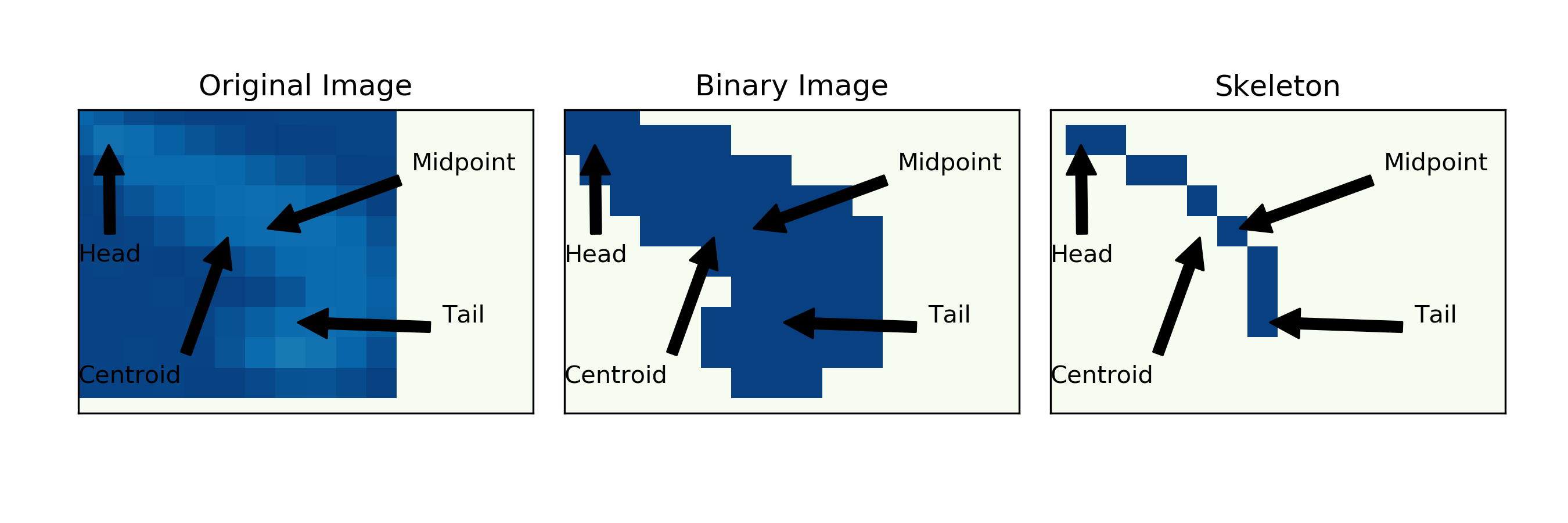
6.6. Visualization of different points on the animal
What exactly do the terms “Centroid” and “Midpoint” mean? I will try to illustrate the difference so that you may choose the appropriate parameter for your experiment:
To identify the animal the tracking algorithm identifies a “blob” that has significantly different pixel intensity values compared to the background.
The centroid is the center of mass (in 2D) of these pixels.
The midpoint is the center of the skeletonized blob.