PiVR has been developed by David Tadres and Matthieu Louis (Louis Lab).

4. Code explanation

Read this guide if you:

1. Want to gain a high-level understanding of how the detection and tracking algorithm work.

2. Do not (yet) want to look into the source code

4.1. Animal detection

The tracking algorithm depends on the approximate location of the animal and a background image in order to identify the animal. The Animal Detection modes (guide, and selection) allow the user to choose between one of three Modes depending on the experimental setup and question asked. (Source Code)

4.1.1. Standard - Mode 1

User perspective:

1. Place animal in the final dish on the arena, taking the optimal image parameters into account

2. Press Start

Behind the scenes:

1. When the user presses Start the camera starts sending pictures to the tracking software.

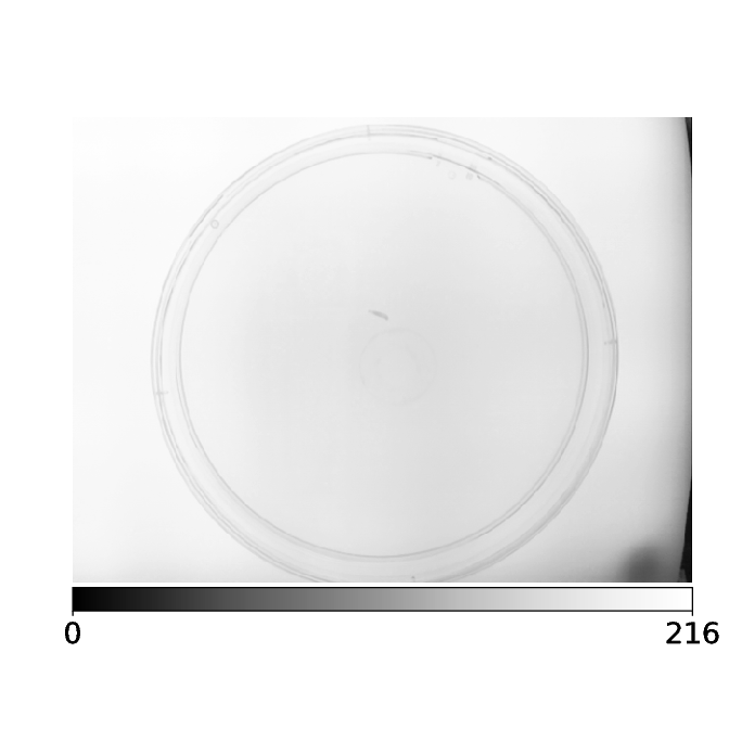
2. For the first frame, the image is just filtered using a gaussian filter with sigma depending on the properties saved in ‘list_of_available_organisms.json’. In short, the sigma will be half the minimal expected cross-section of the animal. Then it takes the next frame.

   

3. Starting with the second frame, the mean of the current and all previously taken images is taken.

   

4. The current frame is then subtracted from the mean of all previous frames

   

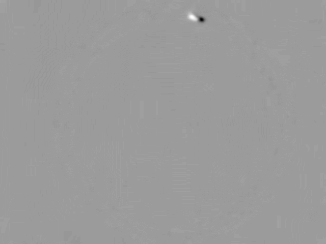
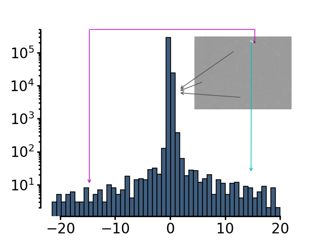
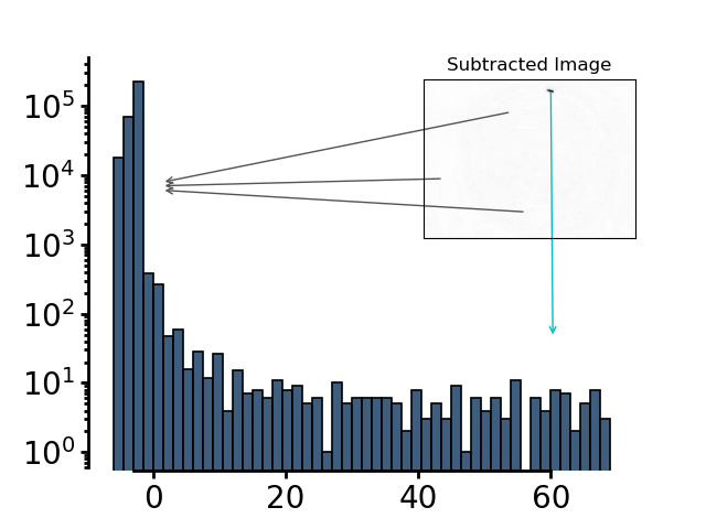
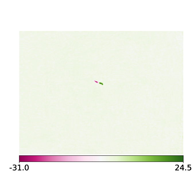
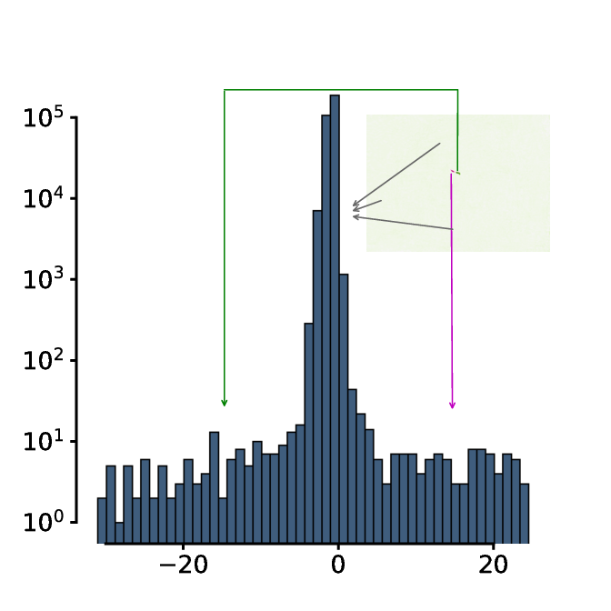
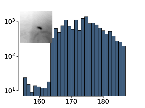
5. The subtracted image has a trimodal distribution of pixels - The main peak is the background (grey arrows). The intensity values for pixels where the animal was before but isn’t anymore has positive values (cyan arrow). The intensity values for the pixels where the animal only recently moved in has negative values (magenta arrow)

   

6. The threshold used to define the animal is subtracting 2 * the standard deviation of the smoothed image from the mean value of pixel intensities

   

7. The current image gets a threshold using the threshold defined above

   

8. Using this binary image, the function label and then the function regionprops of the scikit-image library is applied.

9. Using the filled_area parameter of the regionprops function, the blobs are checked for minimal size defined in the ‘list_of_available_organisms.json’ file for the animal in question. As soon as an image is found where a single blob is larger than the minimal size, the animal counts as being identified.

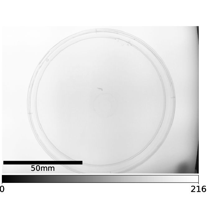
10. The first picture is then filtered again with a gaussian filter with a sigma of 1. This is defined as the background image. This image of course contains the animal as it was at the original position. For many experiments it is unlikely that the animal can be at exactly the same position as in the first frame. If your experiment makes it likely that the animal is in the exact same position more than once, you might want to look at Animal Detection Mode#2 and Mode#3.

    

11. All of this is done in the function pre_experiment.FindAnimal.find_roi_mode_one_and_three()

12. Finally, another frame is taken from the camera. Importantly, the threshold is now calculated locally! This allows for a better separation of the animal and the background by defining a local treshold. The image gets filtered using the local threshold and then subtracted from the first (filtered) image. After applying the label and then the regionprops functions of the scikit-image library the largest blob is defined as the animal. The centroid, the filled area and the bounding box are saved for the tracking algorithm.

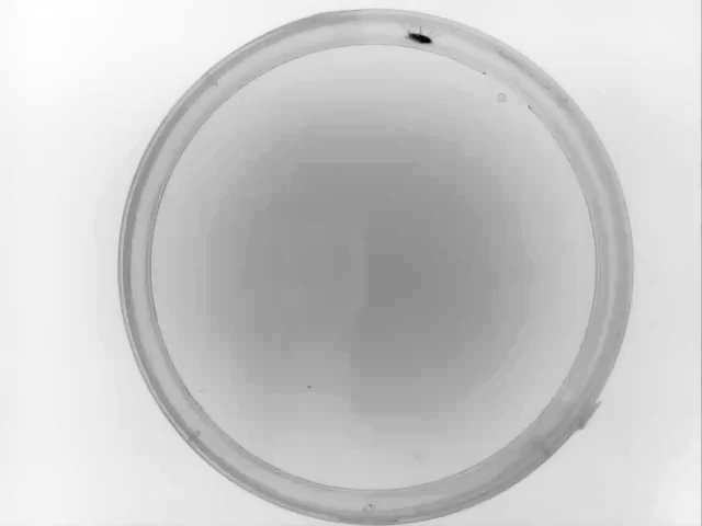
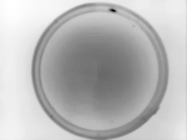
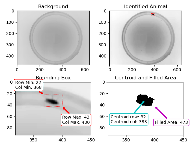
13. Example data collected for this particular example with Animal Detection Mode#1:

    

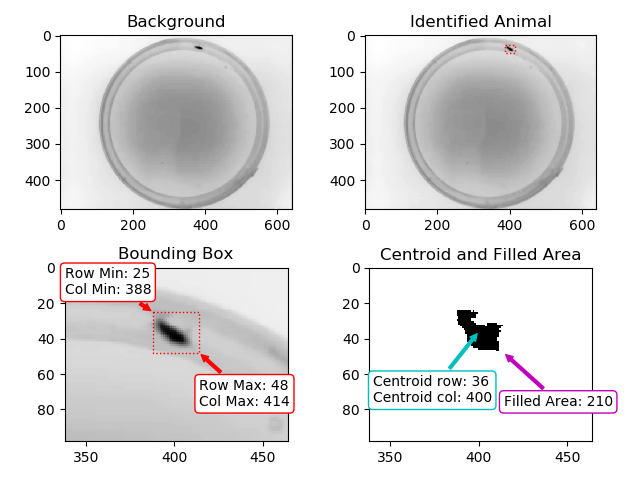
    Result of Animal Detection Mode 1: Top Left: Background image saved for the rest of the experiment. Using Mode 1 the animal will always be present in the background image used during the actual experiment. If this is a problem for your experiment, please check Mode#2 and Mode#3. Top Right: Animal identified during Animal Detection Mode#1. The red box indicates the bounding box of the animal. Bottom Left: Close-up of the detected animal. The bounding box is defined with 4 coordinates: The smallest row (Row Min, or Y-min), the smallest column (Col Min, or X-min), the largest row (Row Max, or Y-max) and the largest column (Col Max, or X-Max). Also see the regionprops function documentation (bbox). Bottom Right: The binary image used by the algorithm to define the animal. The centroid is indicated as well as the filled area. Both parameters are defined using the regionprops function.

14. This is done using: pre_experiment.FindAnimal.define_animal_mode_one()

15. Next, the actual tracking algorithm will be called and run until the experiment is over.

4.1.2. Pre-Define Background - Mode 2

User perspective:

1. Prepare PiVR for the experiment by putting everything except the animal exactly at the position where it will be during the experiment. Take the optimal image parameters into account

2. Press Start

3. User will be asked to take a picture by clicking ‘OK’.

4. Then user will be asked to put the animal without changing anything else in the Field of View of the camera

5. Press Start

Behind the scenes:

1. The image taken without the animal is being used as the background image.

   

2. After the user puts the animal and hits ‘Ok’ the same algorithm as in Mode 1 and 3 is searching for the animal: First a new picture is taken and filtered using a gaussian filter with Sigma = 1:

   

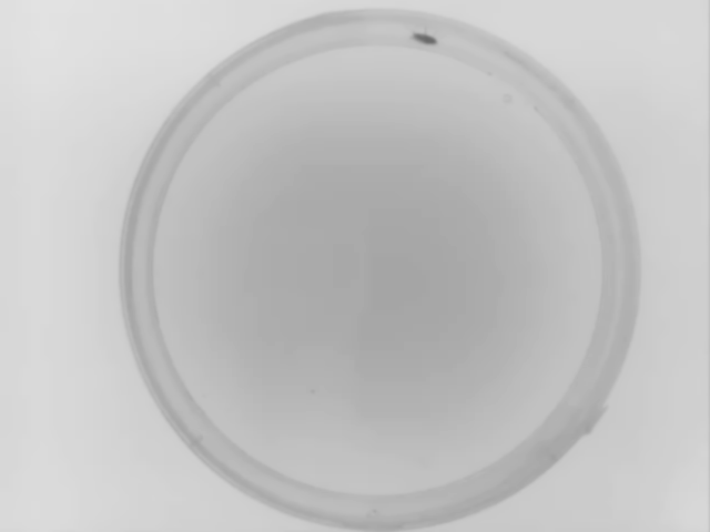
3. This image is subtracted from the background image:

   

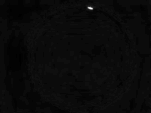
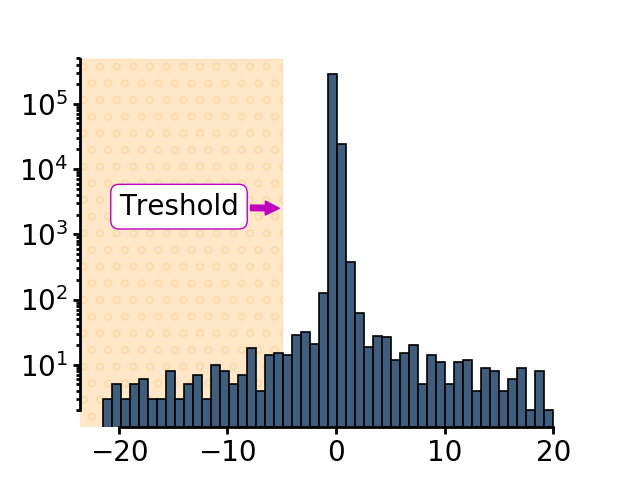
4. The pixel intensity values are a bimodal distribution.

   

5. The threshold is defined as all values larger 2 times the Standard deviation of the the image + the mean pixel intensity values of the image (usually 0)

   

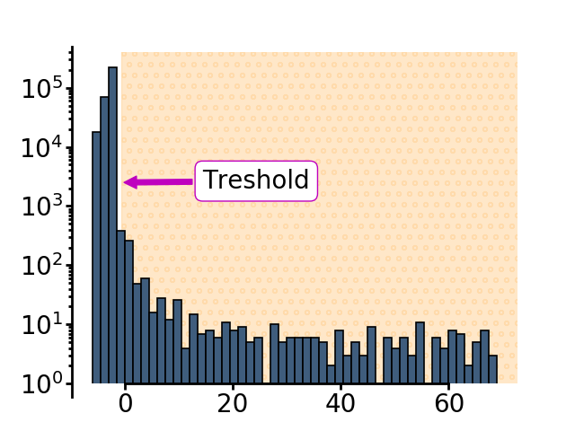
   Threshold to identify animal: On the left the background pixels with a approximate value of zero are seen. Note the logarithmic scale. On the right the yellow rectangle indicates all the pixel intensity values that will count as the identified animal

6. The threshold is used to binarize the image.

   

7. Using this binary image, the function label and then the function regionprops of the scikit-image library is applied.

8. Using the filled_area parameter of the regionprops function, the blobs are checked for minimal size defined in the ‘list_of_available_organisms.json’ file for the animal in question. As soon as an image is found where a single blob is larger than the minimal size, the animal counts as being identified.

9. This is done in pre_experiment.FindAnimal.find_roi_mode_two()

10. Unlike Mode1 it is not necessary to take local thresholding as the animal should be clearly visible compared to the background. The global threshold is used to create a binary image. The largest blob is defined as the animal.

11. Example data collected for this particular example with Animal Detection Mode#2:

    

    Result of Animal Detection Mode 1: Top Left: Background image saved for the rest of the experiment. Top Right: Animal identified during Animal Detection Mode 2. The red box indicates the bounding box of the animal. Bottom Left: Close-up of the detected animal. The bounding box is defined with 4 coordinates: The smallest row (Row Min, or Y-min), the smallest column (Col Min, or X-min), the largest row (Row Max, or Y-max) and the largest column (Col Max, or X-Max). Also see the regionprops function documentation (bbox). Bottom Right: The binary image used by the algorithm to define the animal. The centroid is indicated as well as the filled area. Both parameters are defined using the regionprops function.

12. This is done in pre_experiment.FindAnimal.define_animal_mode_two()

13. Next, the actual tracking algorithm will be called and run until the experiment is over.

4.1.3. Reconstruct Background by Stitching - Mode 3

User perspective:

1. Place animal in the final dish on the arena, taking the optimal image parameters into account

2. Press Start

Behind the scenes:

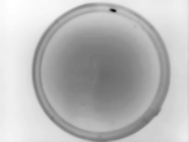
1. As soon as the user hits “Start”, the camera will start streaming images from the camera. Here a fruit fly larva can be seen in the center of the image

   

2. A second image then taken.

   

3. The new image is now subtracted from previous image(s).

   

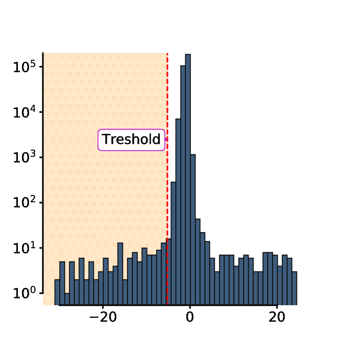
4. The histogram of this image exhibits a trimodal distribution - a very large peak at around 0 indicating all the background pixels, positive pixel intensities indicating coordinates that the animal occupied in the past and has left and negative pixel values indicating coordinates that the animal has not occupied in the first frame but does now.

   

5. The threshold is defined as 4 minus the mean pixel intensity of the subtracted image.

   

6. The threshold is then used to binarize the first image:

   

7. Using this binary image, the function label and then the function regionprops of the scikit-image library is applied.

8. Using the filled_area parameter of the regionprops function, the blobs are checked for minimal size defined in the ‘list_of_available_organisms.json’ file for the animal in question. As soon as an image is found where a single blob is the region of interest in calculated depending on the maximum speed, maximum size and pixel/mm.

   

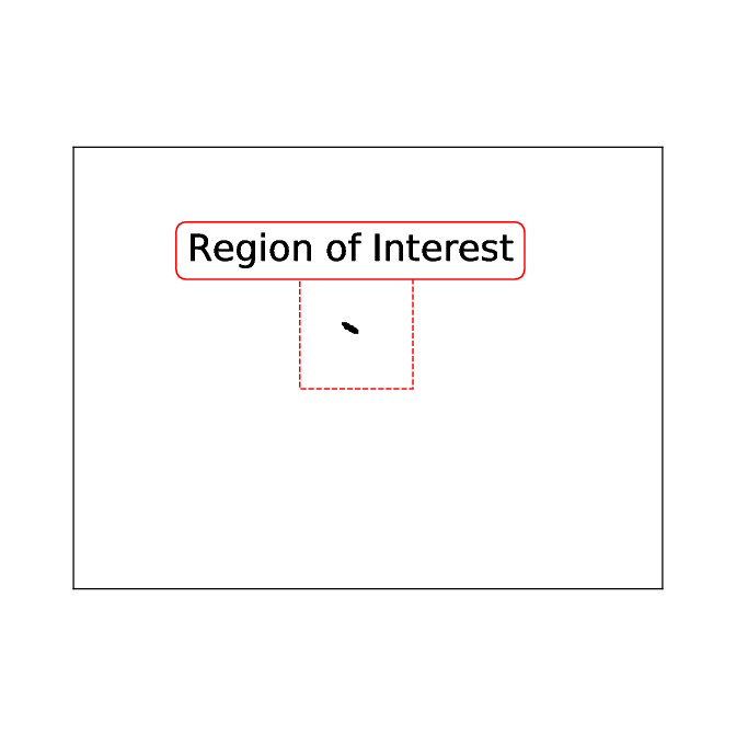
9. So far this has been identical to Mode 1 - both Modes use the identical function up to this point: pre_experiment.FindAnimal.find_roi_mode_one_and_three()

10. Now comes the trickiest part of Mode 3: The animal must be identified as complete as possible. For this the region of interest is used:

    

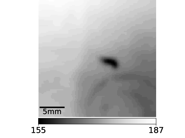
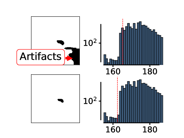
11. The histogram of this region of interest looks very different compared to the histogram of the whole frame. Importantly, the larva now clearly stands out from the background as can be seen in the histogram.

    

12. The threshold is now adjusted until only a single object with animal-like properties is left in the thresholded region of interest. ^

    ^animal like properties are defined in the “list_of_available_organisms.json” file

    

13. It is important to understand the limitations of this approach! This animal identification will only work if the animal is clearly separated from the background. It will not work, for example if the animal is close to the edge of the petri dish, if there are other structures in the arena etc…!

    All this is done using the function: pre_experiment.FindAnimal.define_animal_mode_three()

14. After identifying the animal, the algorithm waits until the animal has left the inital position.

    To do this it will continue capturing images, binarizing them and finally subtracting them from the identfied animal. Only when the original animal is 99.9% reconstructed has the animal left the original position.

    This is done using the function pre_experiment.FindAnimal.animal_left_mode_three()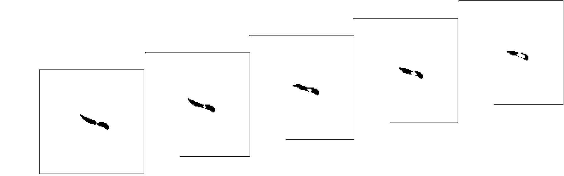

    

15. When the animal has left, the region that was occupied by the animal in the first frame is replaced by the pixels at the same coordinates of the image where the animal has left the original position. This should lead to a “clean” background image, meaning the animal shouldn’t be present (as it would be in Mode 1).

    This is done using the function: pre_experiment.FindAnimal.background_reconstruction_mode_three()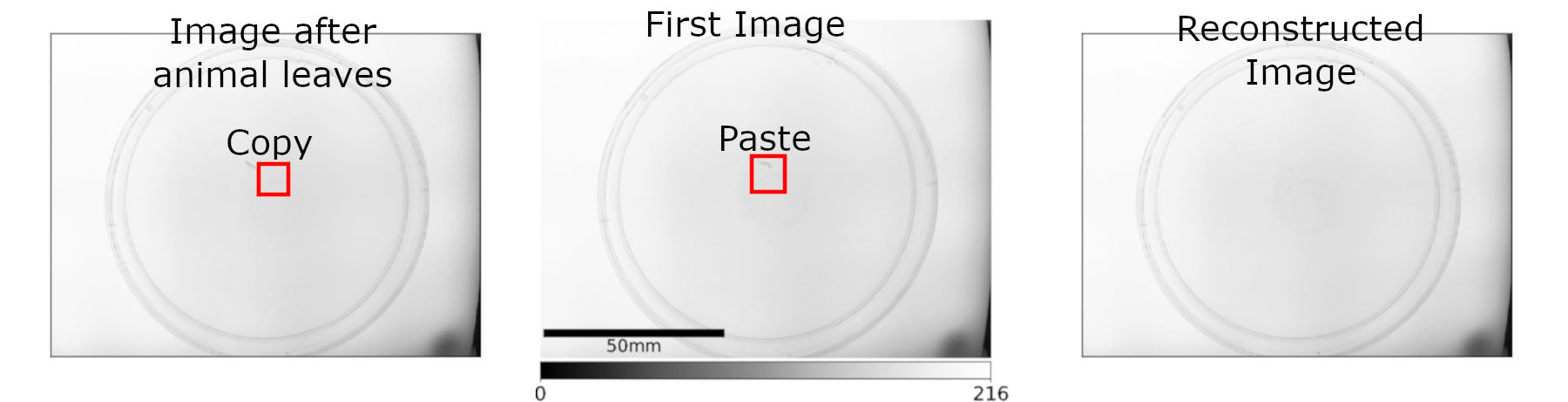

    

16. Before the tracking can start, the location of the animal after background reconstruction must be saved. This is done using the function: pre_experiment.FindAnimal.animal_after_box_mode_three()

4.2. Animal Tracking

After the detection of the animal with any of the described animal detection modes (Mode 1, Mode 2 or Mode 3) the tracking algorithm (fast_tracking.FastTrackingVidAlg.animal_tracking()) starts.

Note

The camera will start recording at the pre-set frame rate. If the frame rate exceed the time it takes for PiVR to process the frame, the next frame will be dropped. For example, if you are recording at 50 frames per second, each frame has to be processed in 20ms (1/50=0.02 seconds). If the frame processing takes 21ms, the next frame is dropped and PiVR will be idle for the next 19ms until the next frame arrives.

1. Once the tracking algorithm starts, the camera and GPU start sending images at the defined frame rate to the CPU, i.e. at 30fps the CPU will receive one new image ever 33ms. Source code here: fast_tracking.FastTrackingControl.run_experiment()

2. The images are then prepared for tracking. Source code here: fast_tracking.FastTrackingVidAlg.write()

3. Next the animal_tracking function which does all the heavy lifting described below is called: fast_tracking.FastTrackingVidAlg.animal_tracking().

4. The Search Box is defined depending on the previous animal position, the selected organism and that organisms specific parameters. For details check source code here: start_GUI.TrackingFrame.start_experiment_function()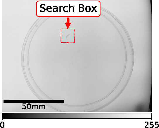

   

5. The content of the Search Box of the current frame is then subtracted from the background frame (generated during animal detection).

   

6. Upon inspection of the histogram of the subtracted image it becomes clear that the animal has clearly different pixel intensity values compared to the background.

   

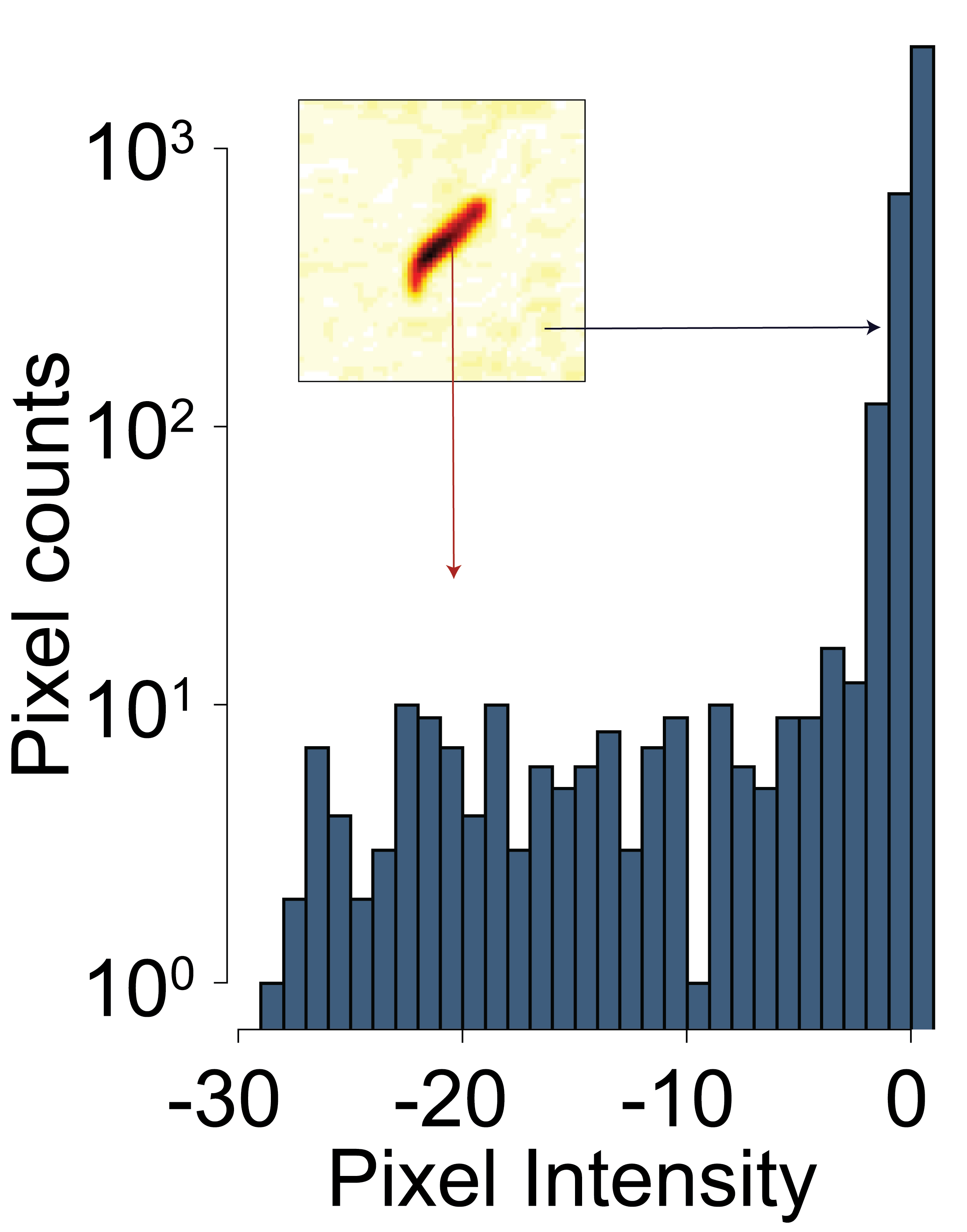
7. The threshold is determined by calculating the mean pixel intensity of the subtracted image and subtracting 3 times the standard deviation.

   

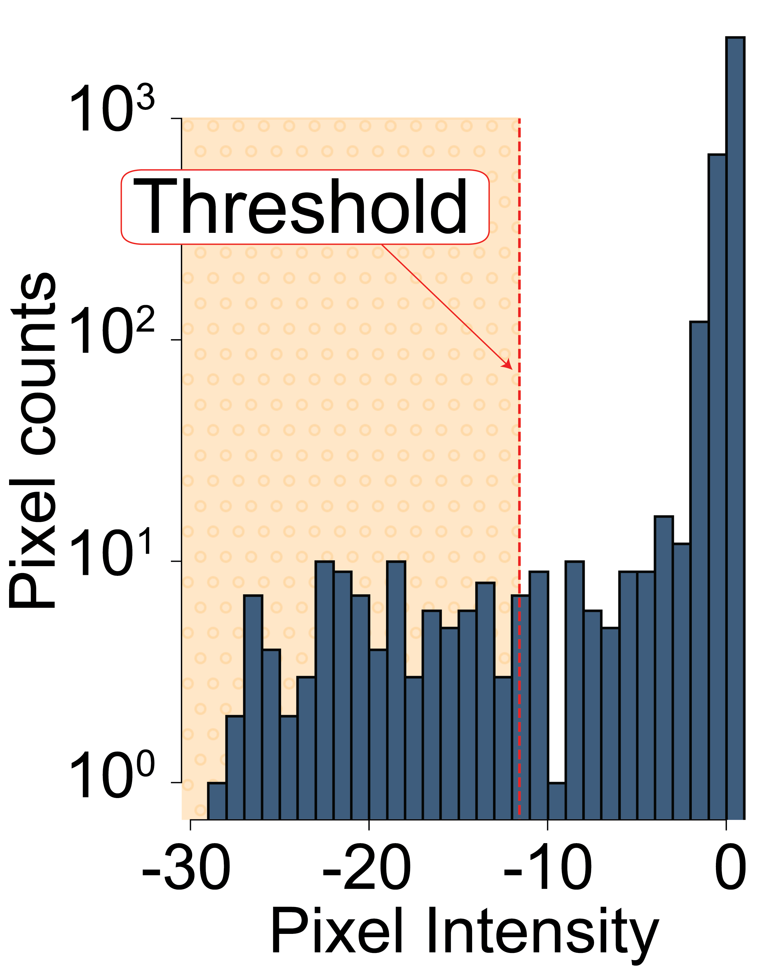
8. This threshold is then used to binarize the current small image:

   

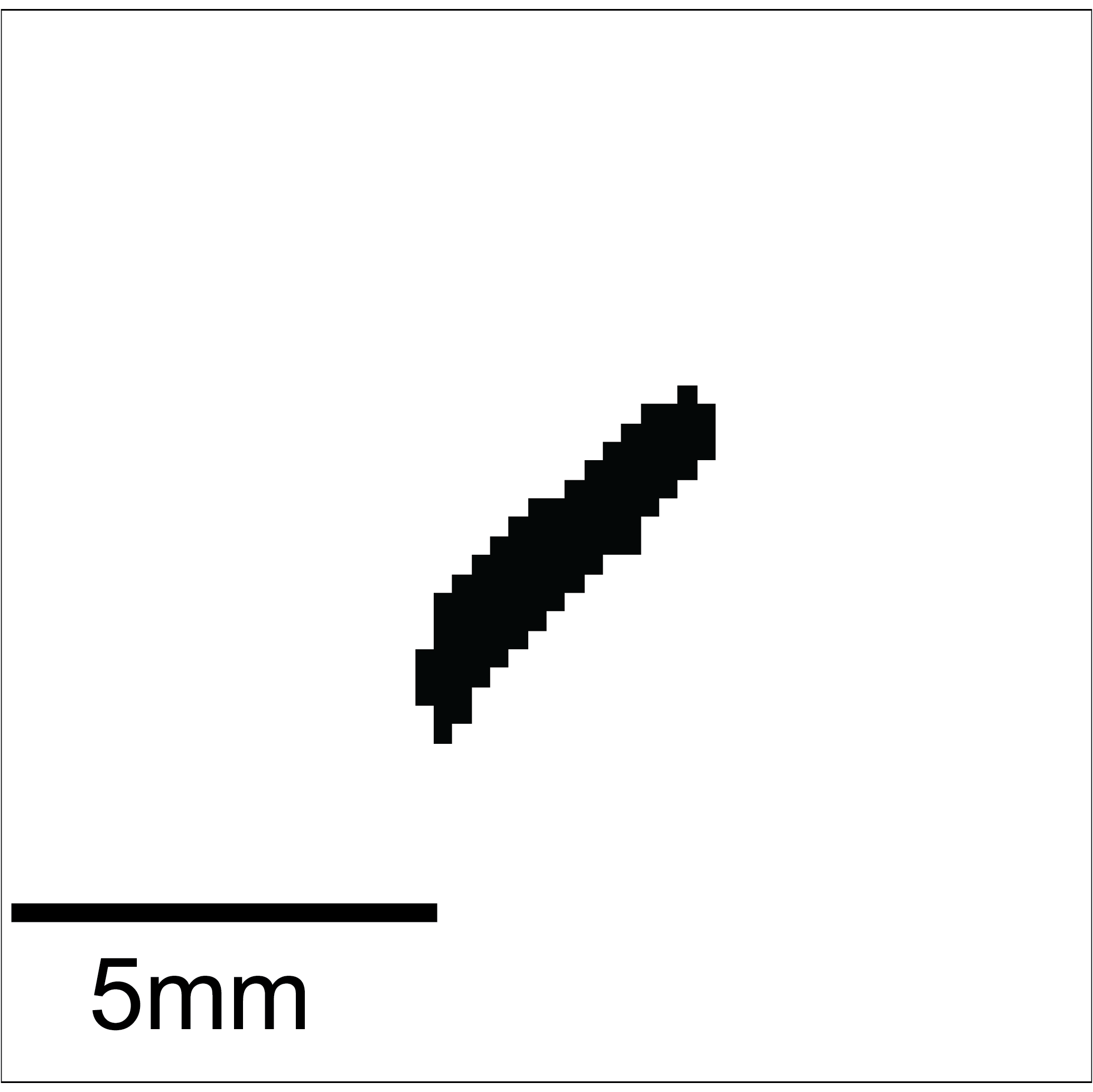
9. Using that binary image, the function label and then the function regionprops of the scikit-image library is applied. This way all ‘blobs’ are identified. Using the animal parameters defined before, the blob that looks the most like the sought after animal is assigned to being the animal.

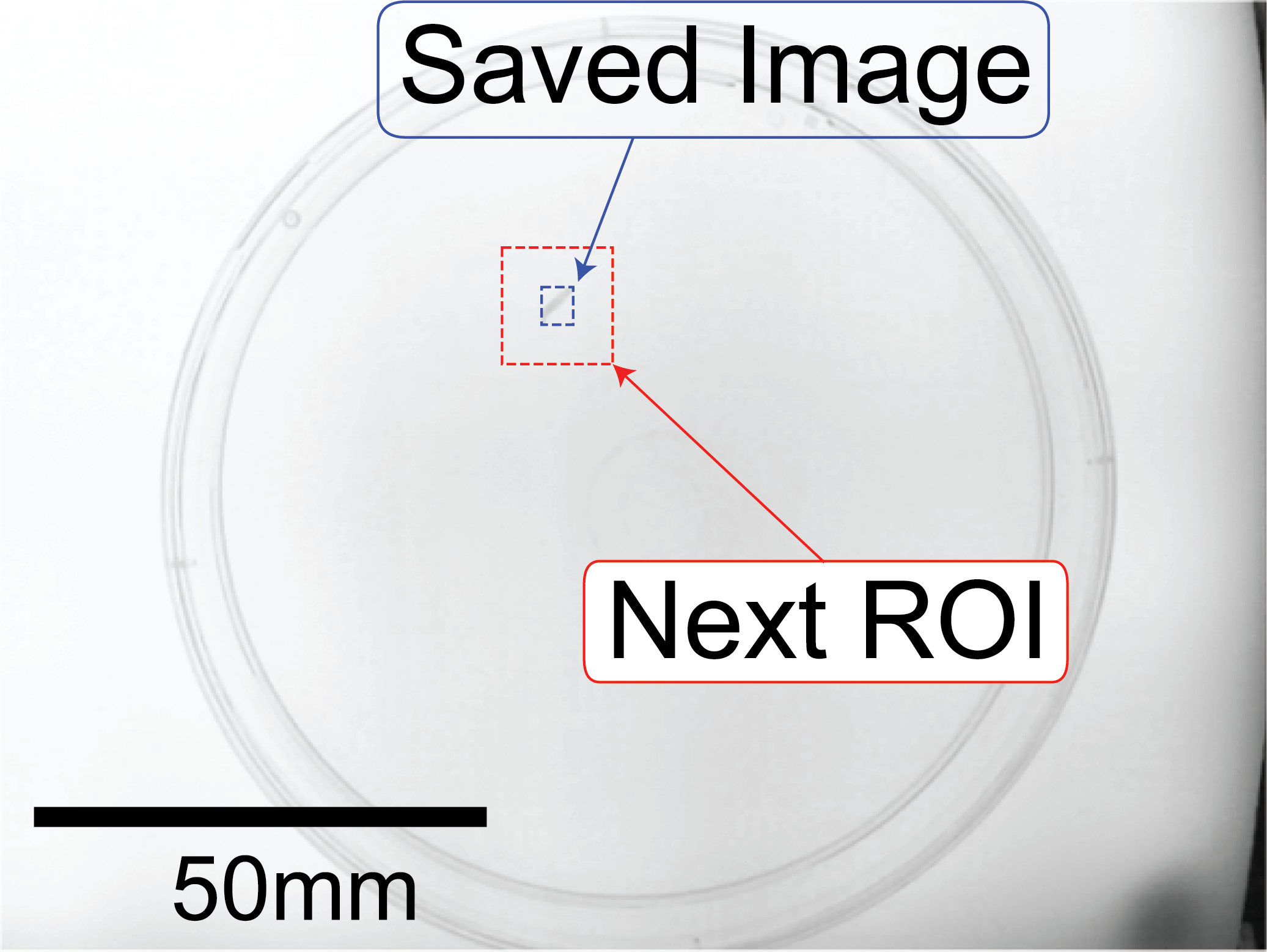
   After detection of the animal, the image of the animal is saved (blue rectangle) and the Search Box for the next frame prepared (red rectangle)

   

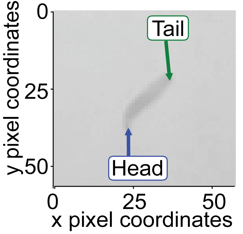
4.3. Head Tail Classification

The Head Tail classification is based upon a Hungarian algorithm.

1. First, the binary image is skeletonized (either with thin function or the skeletonize function)

   

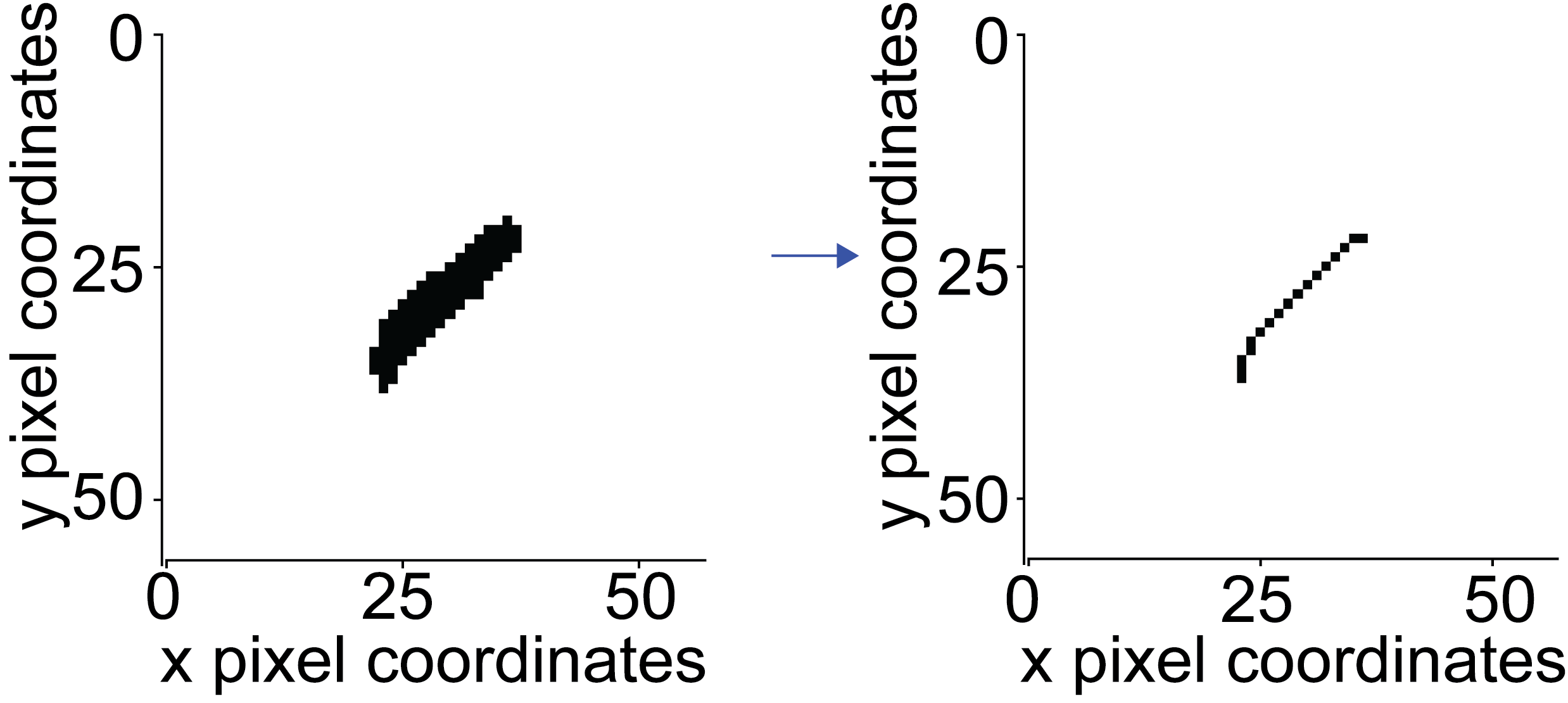
2. Using the rule that the endpoints of that skeleton must only have one neighbour, the endpoints are defined.

   

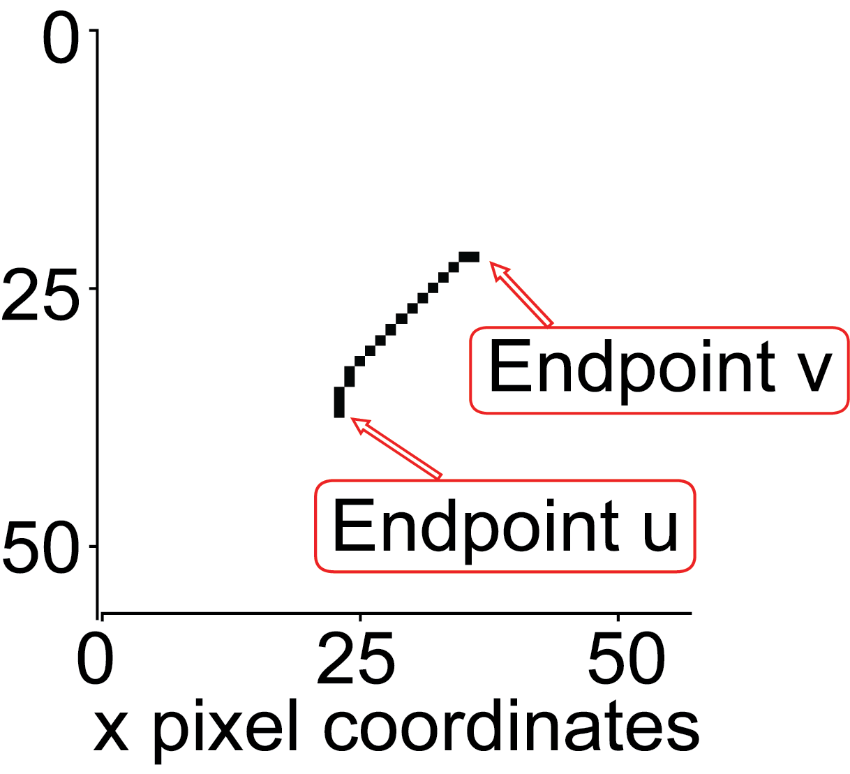
3. To define the head and tail the following conditions must be met:

   1. The aspect ratio of the long axis over the short axis must be at least 1.25

   2. The skeleton must have exactly 2 endpoints

   3. The length of the skeleton must be larger than half the mean length of the previous 3 frames.

4. Next, the distance of each endpoint to a reference point is calculated:

   1. In case the tail has not yet been assigned (happens in the first frame) use the centroid of the previous frame as the reference point.

   2. In case of not having been able to assign a tail in the previous frame, e.g. due to the violation of any of the rules shown above, also use the centroid of the previous frame as the reference point.

   3. Otherwise (in most cases) the endpoint that has been assigned the tail in the previous frame is used as the reference point.

   

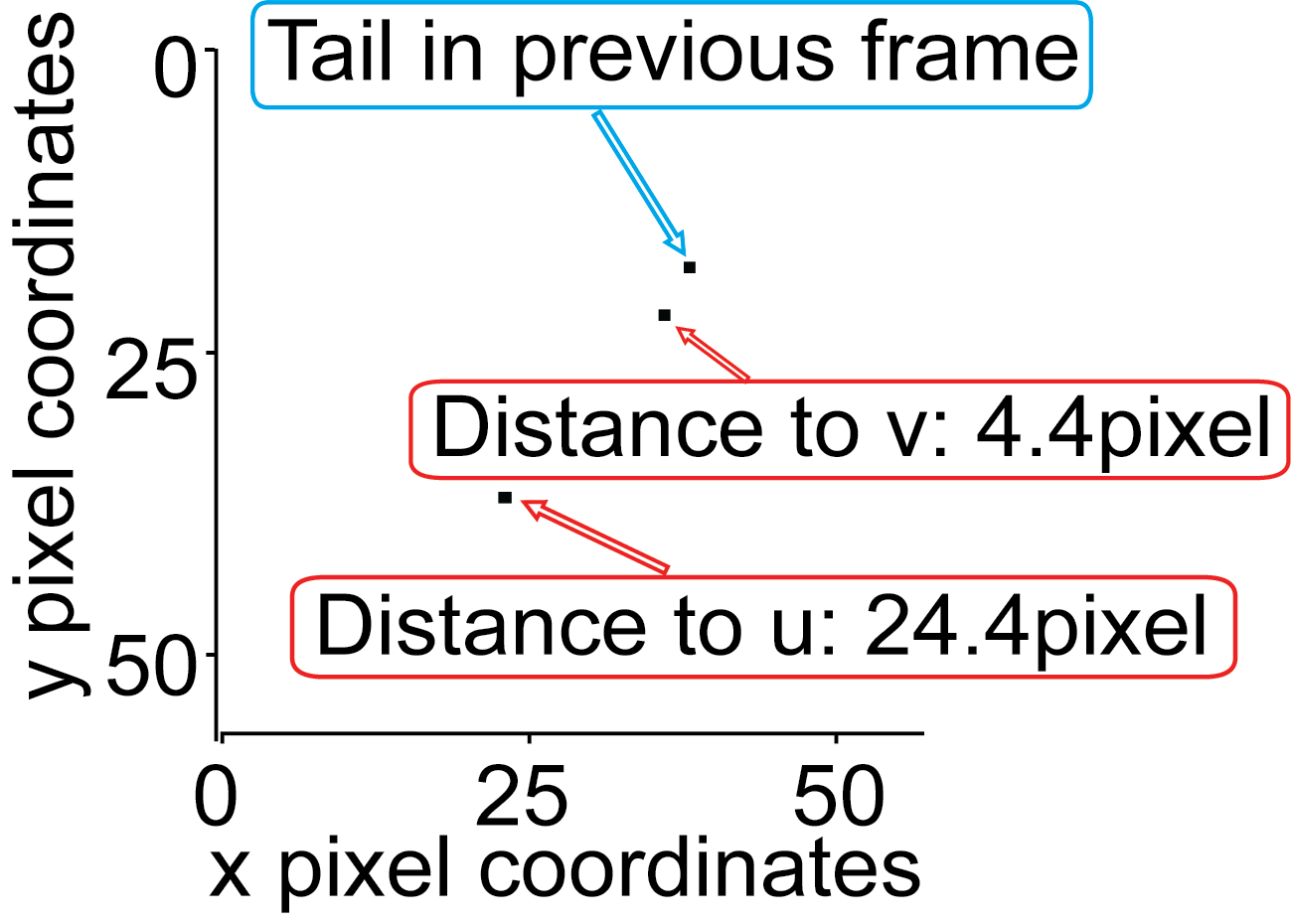
5. Whichever endpoint has the shorter distance the previous reference point is assigned the label ‘Tail’.

   

4.4. Dynamic Virtual Realities

PiVR is capable of presenting virtual realities that change over time, or ‘dynamic virtual realities’. The difference to the ‘standard’ virtual reality is that the dynamic virtual reality will change its stimulus profile over time even if the animal is not moving. See the following move for an application example where a fruit fly larva is tested in a virtual odor plume.

To create such a dynamic virtual reality from scratch, see here.

How does PiVR present such a dynamic virtual reality? The stimulation file is a 3D numpy array with the 3rd dimension coding for time. I will call the virtual arena at a given time slice.

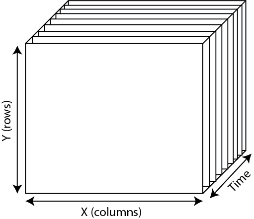
For each timepoint during the experiment, one of the x/y slices is presented to the animal as a virtual arena. How does PiVR know when to update the arena? You could, for example update the arena 15 times per second (Hz), or maybe only once every minute (1Hz).

The relevant parameter is saved directly in the filename of the arena as Hz[xx].npy

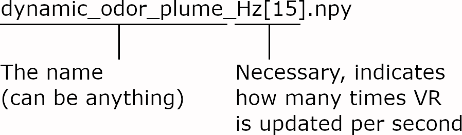
For example, you are running your experiment at 30 frames per second. You want to update the arena 15 times per second. The following pseudo-code will explain how PiVR updates the arena:

# User defined update parameter
recording_framerate = 30 # Hz
dynamic_virtual_reality_update_rate = 15 # Hz
update_VR_every_x_frame = recording_framerate/dynamic_virtual_reality_update_rate
recording_time = 5 # minutes
recording_length = recording_framerate * recording_time * 60
current_VR_time_index = 0

# The for loop indicates a running experiment where PiVR processes
# one frame per iteration
for current_frame in range(recording_length):
    detect_animal_function()
    detect_head_function()

    # Here we update VR according to the update_VR_every_x_frame
    # Note, the modulo operator % returns the remainder of a
    # division. For example 0%2=0, 1%2=1, 2%2=0, 3%2=1 etc.
    if current_frame% update_VR_every_x_frame == 0:
        current_VR_time_index += 1

    # Now, we present the current slice of the virtual reality
    present_VR(stimulation_file[:, :, current_VR_time_index])

    # As the size of the stimulus file in time can be smaller than
    # the length of recording_time the index needs to be reset to
    # zero.
    if current_VR_time_index > size_of_stimulus_file:
        current_VR_time_index = 0

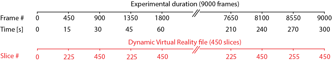
As an example for how this would play out, consider an experiment with the following parameters:

1. Experiment time = 5 minutes (300 seconds)

2. The recording framerate = 30Hz, hence there will be 9000 frames

3. dynamic VR update rate = 15Hz

4. dynamic VR file has 450 time slices.

You can immediately see that there are less slices in the provided stimulus file compared to the other experimental parameters: We want to record for 300 seconds while updating 15 times per second with only 450 slices. We will run out of slices after only 450/15=30 seconds!

PiVR solves this by just starting over at the beginning when it encounters the end of the stimulus file. The figure shown below is visualizing this: