PiVR has been developed by David Tadres and Matthieu Louis (Louis Lab).
8. Advanced topics
8.1. Simulate Real-Time Tracking
Imagine setting up your experiment: preparing the animals, booking the setup/room for a whole afternoon…and then the tracker does not track the animal half of the time!
It is quite frustrating sitting in a dark room trying to troubleshoot these kind of problems.
To alleviate situations like these, there is the option to simulate real time tracking after installing the PiVR software on a PC (=not on the Raspberry Pi).
At the PiVR setup, double check that:
you have set the resolution to resolution you want to use,
that the pixel/mm is set correctly,
that the framerate is identical to the framerate you are trying to achieve with real-time tracking.
that you have selected the correct animal
Then, record a video with these settings. Then record some more.
Transfer the video data to your PC where you have installed the PiVR software and select the Debug->Simulate Online Tracking
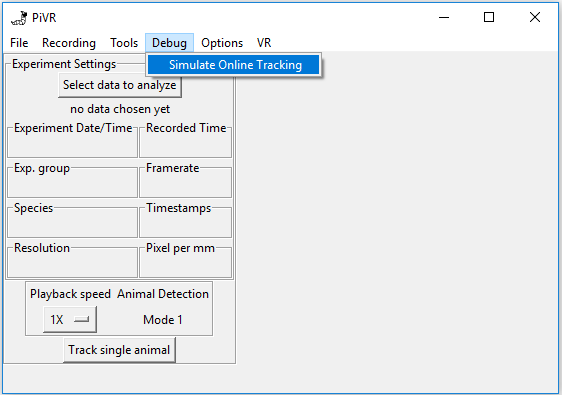
Make sure the Animal Detection Method is the same as the one you want to use during Real-Time tracking.
Note
This has not been tested with Mode 2
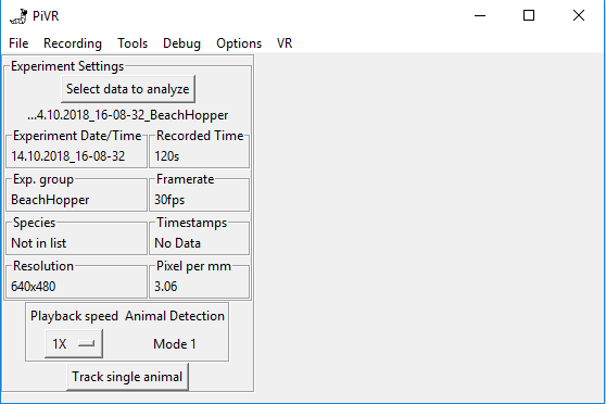
Select a single folder. You will now see the metadata created while the video was taken. Carefully inspect it to see if the settings are as you expect them.
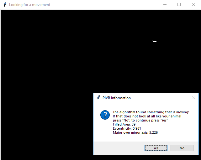
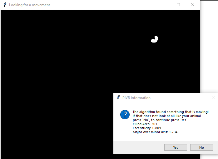
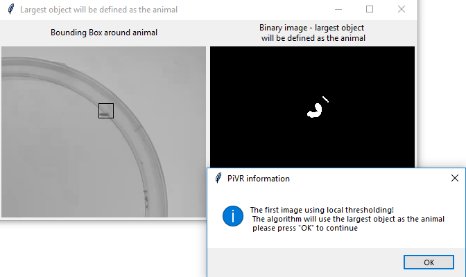
Press the ‘Track Single Animal’ button - you will get a popup as soon as the animal detection algorithm detects a moving object.
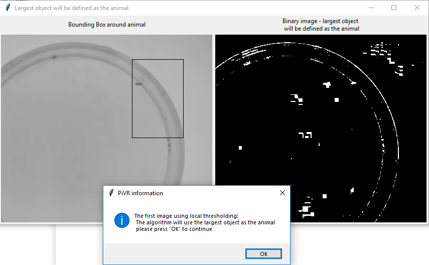
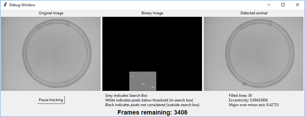
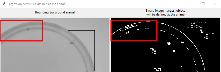
After pressing ok, you will see what the animal detection algorithm has defined as the animal.
It is obvious something has gone wrong here as the image on the right (the binary image) has a lot of spots where the image is white (=areas which are considered to be the animal)
After pressing Ok, the tracking algorithm starts - as the animal has not been properly identified in the first frame, the tracking algorithm is unable to identify the animal during tracking as well:
After going through the simulated tracking, the potential source of the problem has been identified: The animal can not be detected correctly. There are many reasons why this could be:
The edge of the dish seems to have moved a bit during the first couple of frames (red rectangle). If you are able to stabilize the setup to ensure no movement while doing experiments, this problem should be solved.
The fact that several spots in the middle of the dish are wrongly binarized as the potential animal, indicates that the detection algorithm has trouble setting the threshold correctly. This problem arises because the threshold is calculated as 2 standard deviations from the mean of the pixel intensities in the subtracted image
pre_experiment.FindAnimal.define_animal_mode_one(). While the animal is the darkest spot in the image, the whole petri dish is darker than the background which might lead to this problem.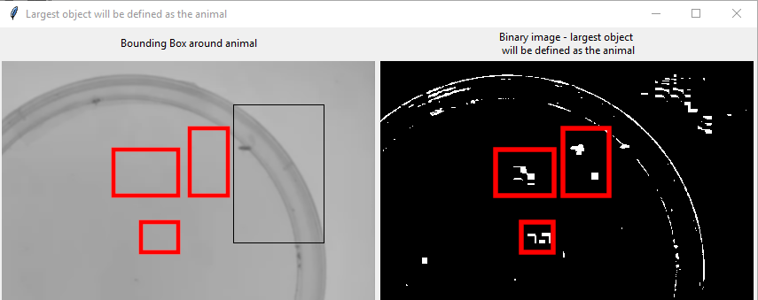
There are two general ways to solve this problem:
Optimize the imaging conditions so that the animal has a higher contrast to the background, which should be as homogenous as possible. See here for an example.
Optimize the animal parameters. You can follow this guide to set stringent animal parameters for tracking.
There are many ways how tracking can fail. Only a single example is described above. I hope the walkthrough will enable you to generally get an idea where during tracking the algorithm fails.
8.2. Tracking of a new animal
PiVR has been used to track a variety of animals: Walking adult fruit flies, fruit fly larvae, spiders, fireflies, pillbugs and zebrafish.
For the tracking algorithm to function optimally, it takes several “animal parameters” into account:
The amount of pixels the animal will fill in the image.
The “roundness” of the animal.
The proportions of the animal.
The length of the animal.
The speed of the animal.
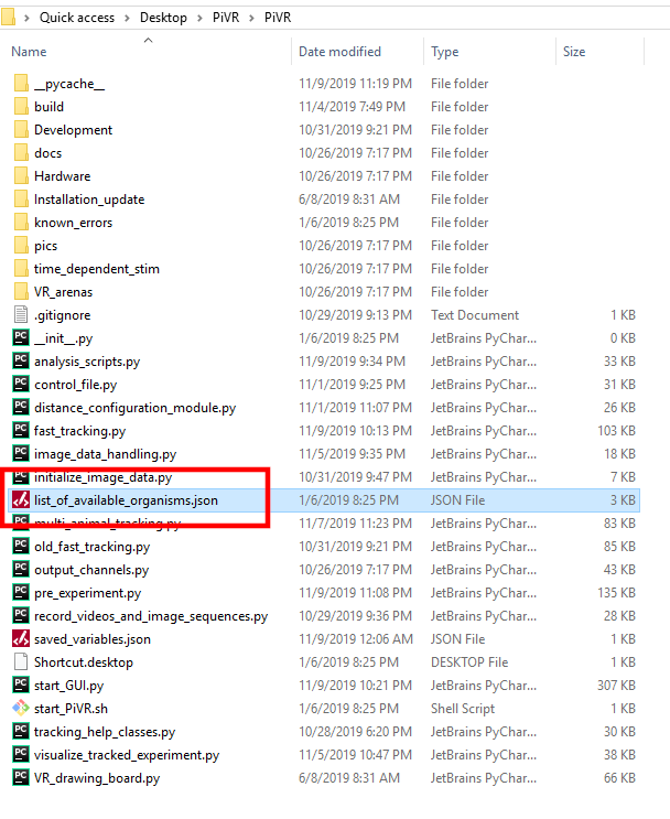
For each animal you can choose in Options->Select Organism these parameters were defined. You can find them in the file “list_of_available_organisms.json” in source code.
If you want to track an animal that is not on the list you can always try to use the “Not in list” option. However, the tracking algorithm might not work optimally.
There is a straightforward pipeline to collect the necessary animal parameters to optimize real-time tracking:
Place your (single!!) animal in the arena you want to use for your experiment.
As always, do not forget to define the pixel/mm.
Select “Not in List” under Options->Select Organism.
Record a video. If you use a fast animal, make sure to select a sufficiently high framerate. As always it is imperative that the camera and the arena are stable during recording, i.e. nothing in the image should move except the animal!
Record for a couple of minutes, i.e. 5 minutes.
Make sure you have videos with animals moving as fast as they might in your actual experiment.
It is also necessary that the animals move for a large fraction of the video!
Take the videos to your PC on which you have installed the PiVR software.
To observe what the algorithm is doing, turn the Debug mode on. This is recommend as you will see immediately if and where something goes wrong. This can help you to solve tracking problems.
Analyze each video using the Tools->Analysis: Single Animal Tracking option.
If using the Debug mode, you will get informed as soon as the algorithm detects an object that is moving. It will also inform you how much space (in pixels) the detected animal occupies, its eccentricity (‘roundness’) and a parameter for proportions (Major axis over minor axis). If the identified object clearly is not the animal answer the question with “No” and the algorithm will look in the next frame the largest moving object.
Next, you will see a side by side comparison of the original picture (with a box drawn around the detected animal and the binary image you have seen in the previous popup.
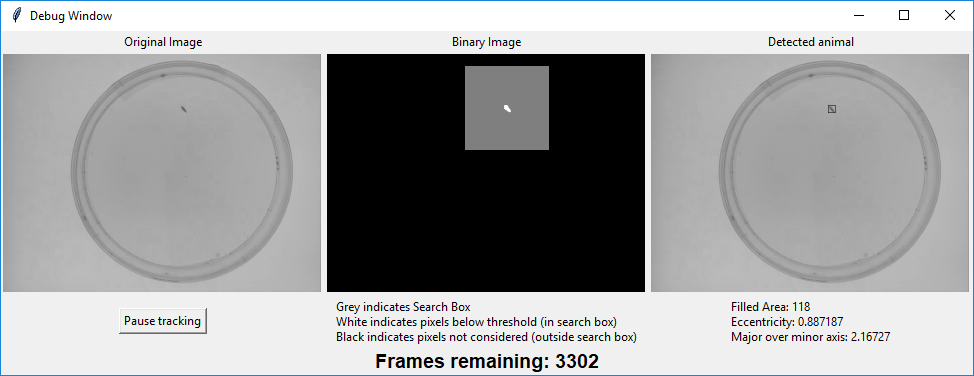
The algorithm will then start tracking. You will see an overview of how the algorithm detects the animal: On the left you can see the original image. In the center you can see the binary image: The grey area indicates the search box (which depends on defined max speed of animal, pixel/mm and framerate) and in white the pixels that are below threshold. The black area is not considered as it is too fare away from the position of the animal in the previous frame. On the right, you can see the result of the tracking: A box drawn around the identified animal. In addition, you can see the animal parameters you are looking for. These are just for your information, read below to see how to comfortably get the list of these parameters.
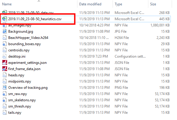
After running the Single Animal Tracking algorithm, you will find a number of new files in each experimental folder. To get to the animal parameters, open the file “DATE_TIME_heuristics.csv”, for example with excel.
Each row in the table stands for one frame. The title of the column describes the value.
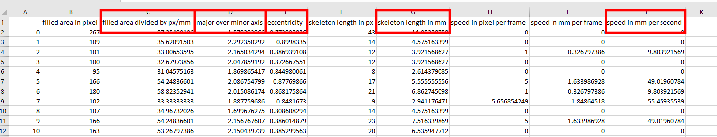
You need to get the following values to get all animal parameters:
A minimum value for filled area (in mm)
A maximum value for filled area (in mm)
A minimum value for eccentricity
A maximum value for eccentricity
A minimum value for major over minor axis
A maximum value for major over minor axis
Maximum skeleton length
Maximum speed of the animal (mm/s)
As the tracking algorithm needs the extreme values to function properly, I have found it easiest to plot a Line Plot for each experiment for each of the relevant parameters. For example for the filled area:
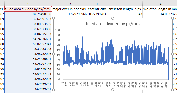
Write down the maximum and minimum value for each of relevant parameters. In this example, the minimum value for filled area in mm would be ~25 and the maximum would be ~90.
Do the same for eccentricity, major over minor axis, skeleton length and maximum speed (mm/s)
Then do the same for a few other videos. The goal is to get extreme values without having to put 0 as minimum and infinity as maximum.
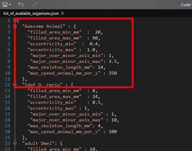
In this example I have found the following parameters:
Minimum value for filled area (in mm): 20
Maximum value for filled area (in mm): 90
Minimum value for eccentricity: 0.4
Maximum value for eccentricity: 1
Minimum value for major over minor axis: 1
Maximum value for major over minor axis: 3.5
Maximum skeleton length: 14
Maximum speed of the animal (mm/s): 350
Now go to the PiVR software folder on your PC and find the file named: “list_of_available_organisms.json”:
Open it with an text editor. I often use “Code Writer” that ships with Windows. You will see that there are repeating structures: A word, defining the name of the animal, then a colon and then some image parameters in brackets.
Note
Json files require correct formatting. Be careful to not accidentally deleting commas etc.

To enter your animal parameters you have two options: The easiest (and safest) option is to choose an animal in the list that you are certain to never use and just enter your parameters:
Alternatively, you may also enter a new “cell” at the end of the list. There is no limit on the number of different animals that can be entered in this list.
Now save the file (do not rename it - If you want to keep a backup, rename the original, i.e. to “list_of_available_organisms_original.json”.)
Restart the PiVR software (so that it reads the newly defined animal parameters).
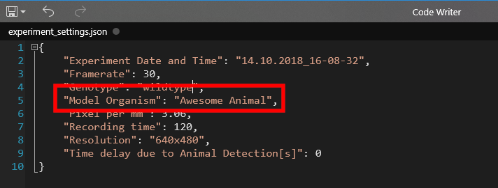
If you want to know whether PiVR is able to perform real-time tracking, you can open the “experiment_settings.json” files in one of the video folders you used to find the animal parameters (or a newly created video) and change the “Model Organism” cell name to your animal name
Now, select the “Debug->Simulate Online Tracking” window, select a video and check whether the algorithm can track the animal in real-time. If not, you might have to select more stringent animal parameters and/or you have to optimize imaging conditions.
8.3. Create your own undistort files
The standard camera introduces a fisheye effect as can be observed below: In reality, the edges of the dish are straight.
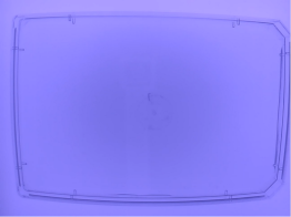
This can lead to problems when collecting data.
PiVR allows for the correction of these optical effects based on a function in the opencv library.
Note
This option can not be turned on if opencv is not installed. If the menu is greyed out make sure to install opencv. In addition, you will have ‘noCV2’ written next to the version number of PiVR.
If you are on the Raspberry Pi the easiest way to install opencv is to wipe the SD card, reinstall the OS and make a clean install of the PiVR software using the PiVR installation file.
On a PC, just install it using conda by first (1) activating the PiVR environment and (2) then entering conda install -c conda-forge opencv
The image below demonstrates the functionality of the undistort algorithm.
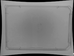
This option is always turned on after v1.7.0 unless you turned it off as described here.
Why is it so important to fix the distorted image? PiVR assigns x and y position of the animal based on the image it gets. If the input image is distorted these values will be off. For example, in the trajectory below the x/y positions of the animal differ visibly between the distorted original image and the undistorted image
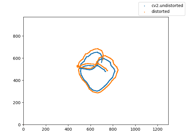
In case of presentation of a virtual reality, the arena gets presented based on the distorted image. This leads to distortion of the virtual reality.
For the undistort algorithm to work, it requires lens-specific distortion coefficients. PiVR comes with these coefficients for the standard lens you get when you buy from the BOM for all standard resolutions (640x480, 1024x768 and 1296x972).
Important
If you are using a different lens you must create your own undistort files. Read on to learn how to do so.
To create your own undistort files please follow the steps below.
Note
You will need to conduct this procedure for every resolution you want to employ in your experiments.
Print this
chessboardon a piece of paper.Go to your PiVR setup and place the printed chessboard on a well lit area (for example the light pad).
Make sure you have selected the resolution you want to use in the future Resolution.
Open the Timelapse Recording Window in the recording menu.
Select a place to save the files. You might want to keep them just in case.
Set it to record for 1 minute with one image every 2 seconds.
Hit start.
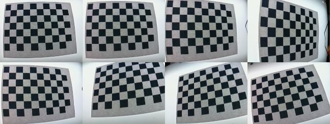
Take the camera into your hands and take images of the chessboard from different angles. See the collage below for an example of the different angles you want to get. Try to get the whole chessboard into the Field of view
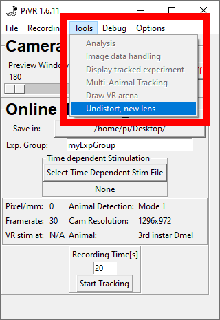
Once you are done, go to ‘Tools’ -> ‘Undistort, new lens’
Press the ‘Chessboard Images’ Button and select the folder where you saved the chessboard images you just took.
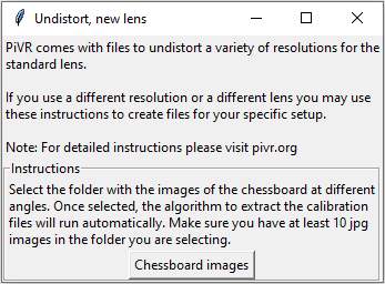
Everything will now freeze for a couple of minutes. At one point you will start to see parts of the chessboard. If the images are not good (e.g. because parts of the chessboard are missing from the field of view) you will get an error message. Please re-take pictures.
Once the algorithm is done, you should have a new set of undistort coefficent files on your local setup. If you want to make a copy, they are in PiVR/PiVR/undistort_matrices/user_provided.
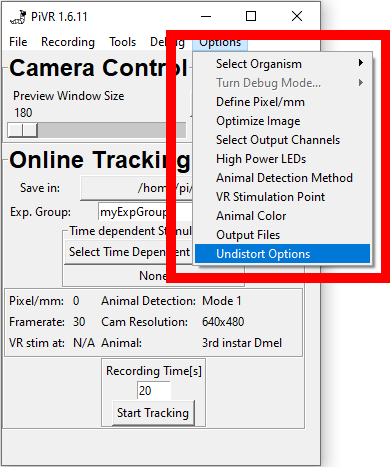
To use these matrices in your next experiment, press the ‘Options’ Menu in the Menu Bar. Then select ‘Undistort Options’.
In the popup select ‘Use your own undistort files’.
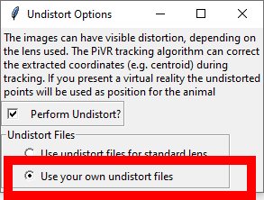
Save the settings.
From now on the output of online tracking is based on your own lens.
8.4. Macro Editor
With v1.8.0 it is now possible to set PiVR up to record several videos consecutively using the new ‘Macro Editor’.
The reason for introducing this option was the experimental need to test a large number of time dependent stimulus files on the same animal to identify the best stimulus for our experiment. This option now allows the experimenter to set up a large number of video recordings which will then be carried out by PiVR without the user having to press ‘Start Video Recording’ after every experiment.
Before you press the ‘Macro Editor’ make sure the following settings are correct as the main PiVR GUI will be frozen while the Macro Editor window is open. (No worries if you forget - there is a save/load option).
The ‘Save in:’ path should point to where you want to save all experiments that are going to be run in the Macro.
Make sure the framerate, resolution and pixel/mm are correct.
You might want to turn the ‘Cam On’ now however it might be hard to see the macro editor if the Preview Window Size is too large.
After pressing the ‘Macro Editor’ button (only accessible on a PiVR setup) a new window opens:

On the left hand side are the options to create a new series of recordings:
‘Load Macro’ allows one to select a previously created (and saved) macro.
‘Add Experiment’ adds an experiment.
‘Delete Experiment’ removes the last Experiment.

Note the following:
You can only select a Time Dependent Stimulus File for the last experiment (red circle).
You don’t have to select a Time Dependent Stimulus File (red rectangle).
You can leave the ‘Exp. Group’ empty. The experimental folder will then just be the date and time of when the experiment was run (and whatevery ou put into the ‘common string’ field.
Avoid ‘.’ in the common string.
You can now save the Macro if you plan on using it again.
Note that the estimate Total Macro Duration is shown on the right hand side.
Note
This ‘Total Macro Duration’ is a lower limit as it doesn’t account for time it takes to save the video and write other datafiles. But it should give a reasonable estimate.
Once the Macro is set up, press ‘Start Macro’.
Since a Macro can take a significant amount of time there is a progress indicator:

A video recording that has finished is indicated with a green ‘Exp #’ while recordings that have not yet finished are indicated in red.